pytorch系列6 -- activation_function 激活函数 relu, leakly_relu, tanh, sigmoid及其优缺点
主要包括:
- 为什么需要非线性激活函数?
- 常见的激活函数有哪些?
- python代码可视化激活函数在线性回归中的变现
- pytorch激活函数的源码
为什么需要非线性的激活函数呢?
只是将两个或多个线性网络层叠加,并不能学习一个新的东西,接下来通过简单的例子来说明一下:
假设
- 输入 x x x
- 第一层网络参数: w 1 = 3 , b 1 = 1 w_1 = 3, b_1=1 w1=3,b1=1
- 第二层网络参数: w 2 = 2 , b 2 = 2 w_2=2, b_2=2 w2=2,b2=2
经过第一层后输出为 y 1 = 3 × x + 1 y_1 = 3\times x + 1 y1=3×x+1经过第二层后的输出为: y 2 = 2 × y 1 + 2 = 2 × ( 3 × x + 1 ) + 2 = 6 × x + 4 y_2=2\times y_1 +2 = 2\times(3\times x+ 1) + 2=6 \times x +4 y2=2×y1+2=2×(3×x+1)+2=6×x+4
是不是等同于一层网络: w = 6 , b = 4 w=6,b=4 w=6,b=4
所以说简单的堆叠网络层,而不经过非线性激活函数激活,并不能学习到新的特征学到的仍然是线性关系。
接下来看一下经过激活函数呢?
仍假设
- 输入 x x x
- 第一层网络参数: w 1 = 3 , b 1 = 1 w_1 = 3, b_1=1 w1=3,b1=1
- 经过激活函数Relu: f ( x ) = m a x ( 0 , x ) f(x)=max(0, x) f(x)=max(0,x)
- 第二层网络参数: w 2 = 2 , b 2 = 2 w_2=2, b_2=2 w2=2,b2=2
通过激活函数的加入可以学到非线性的关系,这对于特征提取具有更强的能力。接下来结合函数看一下,输入的 x x x在经过两个网络后的输出结果:
# -*- coding: utf-8 -*-
"""
Spyder Editor

This is a temporary script file.
"""


import matplotlib.pyplot as plt
import numpy as np
x = np.arange(-3,3, step=0.5)

def non_activation_function_model(x):
    y_1 = x * 3 + 1
    y_2 = y_1 * 2 + 2
    print(y_2)

    return y_2


def activation_function_model(x):
    y_1 = x * 3 + 1
    y_relu =np.where( y_1 > 0,  y_1, 0)
    # print(y_relu)

    y_2 = y_relu * 2 + 1
    print(y_2)

    return y_2


y_non = non_activation_function_model(x)

y_ = activation_function_model(x)


plt.plot(x, y_non, label='non_activation_function')
plt.plot(x, y_, label='activation_function')
plt.legend()
plt.show()
out:

可以看出,通过激活函数,网络结构学到了非线性特征,而不使用激活函数,只能得到学到线性特征。
常用的激活函数有:
- Sigmoid
- Tanh
- ReLU
- Leaky ReLU
分式函数的求导函数: ( g ( x ) f ( x ) ) ′ = g ( x ) ′ f ( x ) − g ( x ) f ( x ) ′ f ( x ) 2 (\frac{g(x)}{f(x)})^{'} = \frac{g(x)^{'}f(x)-g(x)f(x)^{'}}{f(x)^2} (f(x)g(x))′=f(x)2g(x)′f(x)−g(x)f(x)′
- Sigmoid函数
σ ( x ) = 1 1 + e − x \sigma(x) = \frac{1}{1+e^{-x}} σ(x)=1+e−x1
其导函数为: d σ ( x ) / d x = σ ( x ) ( 1 − σ ( x ) ) d\sigma(x)/dx = \sigma(x)(1-\sigma(x)) dσ(x)/dx=σ(x)(1−σ(x))
两者的函数图像:
import numpy as np
import matplotlib.pyplot as plt

def sigma(x):
    return 1 / (1 + np.exp(-x))

def sigma_diff(x):
    return sigma(x) * (1 - sigma(x))

x = np.arange(-6, 6, step=0.5)
y_sigma = sigma(x)
y_sigma_diff = sigma_diff(x)
axes = plt.subplot(111)
axes.plot(x, y_sigma, label='sigma')
axes.plot(x, y_sigma_diff, label='sigma_diff')
axes.spines['bottom'].set_position(('data',0))
axes.spines['left'].set_position(('data',0))
axes.legend()
plt.show()

优点:
-
是便于求导的平滑函数;
-
能压缩数据,保证数据幅度不会趋于 + ∞ 或 − ∞ +\infin或-\infin +∞或−∞
缺点:
-
容易出现梯度消失(gradient vanishing)的现象:当激活函数接近饱和区时,变化太缓慢,导数接近0,根据后向传递的数学依据是微积分求导的链式法则,当前导数需要之前各层导数的乘积,几个比较小的数相乘,导数结果很接近0,从而无法完成深层网络的训练。
-
Sigmoid的输出均值不是0(zero-centered)的:这会导致后层的神经元的输入是非0均值的信号,这会对梯度产生影响。以 f=sigmoid(wx+b)为例, 假设输入均为正数(或负数),那么对w的导数总是正数(或负数),这样在反向传播过程中要么都往正方向更新,要么都往负方向更新,使得收敛缓慢。
-
指数运算相对耗时
- tanh函数
t a n h ( x ) = e x − e − x e x + e − x tanh(x)=\frac{e^x-e^{-x}}{e^x+e^{-x}} tanh(x)=ex+e−xex−e−x
其导函数: d ( t a n h ( x ) ) / d x = 4 ( e x + e − x ) 2 d(tanh(x))/dx=\frac{4}{(e^x+e^{-x})^2} d(tanh(x))/dx=(ex+e−x)24
两者的函数图像:
import numpy as np
import matplotlib.pyplot as plt


def tanh(x):
    return (np.exp(x) - np.exp(-x)) / (np.exp(x) + np.exp(-x))

def tanh_diff(x):
    return 4 / np.power(np.exp(x) + np.exp(-x), 2)

x = np.arange(-6, 6, step=0.5)
y_sigma = tanh(x)
y_sigma_diff = tanh_diff(x)
axes = plt.subplot(111)
axes.plot(x, y_sigma, label='sigma')
axes.plot(x, y_sigma_diff, label='sigma_diff')
axes.spines['bottom'].set_position(('data',0))
axes.spines['left'].set_position(('data',0))
axes.legend()
plt.show()
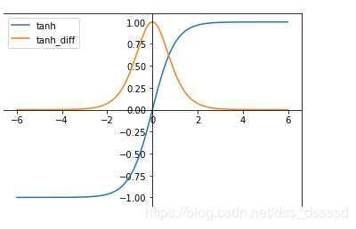
tanh函数将输入值规范到[-1,1],并且输出值的平均值为0,解决了sigmoid函数non-zero问题。但与sigmoid相同的是也存在梯度消失和指数运算的缺点
- Relu函数 :在全区间上不可导
R e l u ( x ) = m a x ( 0 , x ) Relu(x) = max(0, x) Relu(x)=max(0,x)
其导数为:
f ( x ) = { 0 , if x < 0 1 , e l s e f(x) = \begin{cases} 0, & \text{if $x < 0$ } \\ 1, & \text else \end{cases} f(x)={0,1,if x<0 else
其函数图像为:
import numpy as np
import matplotlib.pyplot as plt


def relu(x):
    return np.where(x > 0, x, 0)

def relu_diff(x):
    return np.where(x > 0, 1, 0 )
x = np.arange(-6, 6, step=0.01)
y_sigma = relu(x)
y_sigma_diff = relu_diff(x)
axes = plt.subplot(111)
axes.plot(x, y_sigma, label='sigma')
axes.plot(x, y_sigma_diff, label='sigma_diff')
axes.spines['bottom'].set_position(('data',0))
axes.spines['left'].set_position(('data',0))
axes.legend()
plt.show()

优点:
- 收敛速度明显快于sigmoid和tanh
- 不存在梯度消失问题
- 计算复杂度低,不需要指数运算
缺点:
-
Relu输出的均值非0
-
存在神经元坏死现象(Dead ReLU Problem),某些神经元可能永远不会被激活,导致相应参数永远不会被更新(在负数部分,梯度为0)
产生这种现象的原因 有两个:
- 参数初始化问题: 采用Xavier初始化方法,使的输入值和输出值的方差一致
- 学习率learning_rate太大,导致参数更新变化太大,很容易使得输出值从正输出变成负输出。:设置较小的learning_rate,或者使用学习率自动调节的优化算法
-
relu不会对数据做规范化(压缩)处理,使得数据的幅度随模型层数的增加而不断增大
- Leakly ReLU
f ( x ) = m a x ( 0.01 x , x ) f(x)=max(0.01x, x) f(x)=max(0.01x,x)
其导函数为:
f ( x ) = { 0.01 , if x < 0 1 , e l s e f(x) = \begin{cases} 0.01, & \text{if $x < 0$ } \\ 1, & \text else \end{cases} f(x)={0.01,1,if x<0 else
函数图像:
import numpy as np
import matplotlib.pyplot as plt

def lea_relu(x):
   return np.array([i if i > 0 else 0.01*i for i in x ])


def lea_relu_diff(x):
    return np.where(x > 0, 1, 0.01)

x = np.arange(-6, 6, step=0.01)
y_sigma = lea_relu(x)
y_sigma_diff = lea_relu_diff(x)
axes = plt.subplot(111)
axes.plot(x, y_sigma, label='lea_relu')
axes.plot(x, y_sigma_diff, label='lea_relu_diff')
axes.spines['bottom'].set_position(('data',0))
axes.spines['left'].set_position(('data',0))
axes.legend()
plt.show()
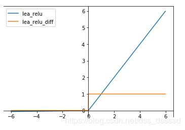
此激活函数的提出是用来解决ReLU带来的神经元坏死的问题,可以将0.01设置成一个变量a,其中a可以由后向传播学习。但是其表现并不一定比ReLU好
以上上述四种激活函数基本是常用的激活函数,现在最常用的激活函数是Relu
具有收敛速度快的优点,但必须要设置较低的学习率和好的参数初始化
接下来通过代码看一下四种激活函数在线性回归中的表现:
# -*- coding: utf-8 -*-
"""
Spyder Editor

This is a temporary script file.
"""


import matplotlib.pyplot as plt
import numpy as np
x = np.arange(-1,1, step=0.01)

def model(x, activation=None):
    y_1 = x * 3 + 0.1
    if  activation:
        y_1 = activation(y_1)
    return y_1 * 2 +0.2


y_non = model(x)

y_1 = model(x, activation=relu)
y_2 = model(x, activation=sigma)
y_3 = model(x, activation=tanh)
y_4 = model(x, activation=lea_relu)


plt.plot(x, y_non, label='non_activation_function')
plt.plot(x, y_1, label='relu')
plt.plot(x, y_2, label='sigmoid')
plt.plot(x, y_3, label='tanh')
plt.plot(x, y_4, label='leakly_relu')
plt.legend()
plt.show()

def relu(x):
    return np.where(x>0, x, 0)
def sigma(x):
    return 1 / (1 + np.exp(-x))
def tanh(x):
    return (np.exp(x) - np.exp(-x)) / (np.exp(x) + np.exp(-x))

def lea_relu(x):
    return np.array([i if i > 0 else 0.01*i for i in x ])
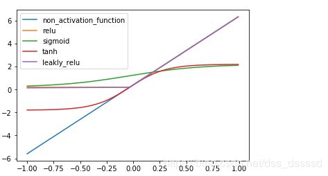
可以看出relu,sifmoid和tanh都表现出了非常好的非线性的关系。
看一下pytorch实现
所有的非线性激活函数:
https://pytorch.org/docs/stable/nn.html#non-linear-activations-weighted-sum-nonlinearity
基类都是nn.Module, 都实现__call__和forward。
nn.ReLU
https://pytorch.org/docs/stable/nn.html#torch.nn.ReLUnn.LeakyReLU(negative_slope=0.01, inplace=False)
https://pytorch.org/docs/stable/nn.html#torch.nn.LeakyReLUnn.sigmoid
https://pytorch.org/docs/stable/nn.html#torch.nn.Sigmoidnn.tanh
https://pytorch.org/docs/stable/nn.html#torch.nn.Tanh