自编码实现浅层神经网络

简介

不使用python神经网络相关库，自行编码实现浅层神经网络。其中隐藏层设置了4个unit。相关可参考Andrew NG 的深度学习课程。

1 - Packages¶

# Packages import
import numpy as np
import matplotlib.pyplot as plt
import sklearn.datasets

%matplotlib inline

2 - Dataset

def load_extra_datasets():  
    N = 200
    noisy_circles = sklearn.datasets.make_circles(n_samples=N, factor=.5, noise=.3)
    noisy_moons = sklearn.datasets.make_moons(n_samples=N, noise=.2)
    blobs = sklearn.datasets.make_blobs(n_samples=N, random_state=5, n_features=2, centers=6)
    gaussian_quantiles = sklearn.datasets.make_gaussian_quantiles(mean=None, cov=0.5, n_samples=N, n_features=2, n_classes=2, shuffle=True, random_state=None)
    no_structure = np.random.rand(N, 2), np.random.rand(N, 2)
    
    return noisy_circles, noisy_moons, blobs, gaussian_quantiles, no_structure

# Datasets
noisy_circles, noisy_moons, blobs, gaussian_quantiles, no_structure = load_extra_datasets()

datasets = {"noisy_circles": noisy_circles, 
            "noisy_moons": noisy_moons,
            "blobs": blobs, 
            "gaussian_quantiles": gaussian_quantiles}
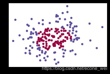
dataset = "gaussian_quantiles"
X, Y = datasets[dataset]
X = X.T;  Y = Y.reshape(1, Y.size);

# make blobs binary
if dataset == blobs:
    Y = Y%2
    
# Visualize the data
plt.scatter(X[0, :],X[1, :], c = Y.reshape(-1,), s = 40, cmap = plt.cm.Spectral)

3 - Neural Network model(背景知识)

Logistic regression did not work well on the “flower dataset”. You are going to train a Neural Network with a single hidden layer.

Here is our model:

Mathematically:

For one example $x^{(i)}$:
$$z^{[1](i)}=W^{[1]}{x}^{(i)}+b^{[1](i)}\text{\hspace{1em}(1)}$$
$$a^{[1](i)}=\tanh (z^{[1](i)})\text{\hspace{1em}(2)}$$
$$z^{[2](i)}=W^{[2]}{a}^{[1](i)}+b^{[2](i)}\text{\hspace{1em}(3)}$$
$${\hat{y}}^{(i)}=a^{[2](i)}=\sigma (z^{[2](i)})\text{\hspace{1em}(4)}$$
$$y_{prediction}^{(i)}=\{\begin{array}{ll}1& if{a}^{[2](i)}>0.5\\ 0& otherwise\end{array}\text{\hspace{1em}(5)}$$

Given the predictions on all the examples, you can also compute the cost $J$ as follows:
$$J=-\frac{1}{m}\sum _{i=0}^m\left(y^{(i)}\log \left(a^{[2](i)}\right)+(1-y^{(i)})\log \left(1-a^{[2](i)}\right)\right)\text{\hspace{1em}(6)}$$

Reminder: The general methodology to build a Neural Network is to:
1. Define the neural network structure ( # of input units, # of hidden units, etc).
2. Initialize the model’s parameters
3. Loop:
- Implement forward propagation
- Compute loss
- Implement backward propagation to get the gradients
- Update parameters (gradient descent)

You often build helper functions to compute steps 1-3 and then merge them into one function we call nn_model(). Once you’ve built nn_model() and learnt the right parameters, you can make predictions on new data.

---

主要实现步骤

3.1 - Defining the neural network structure

3.2 - Initialize the model’s parameters

3.3 - The Loop（forward propagation、backward propagation、compute Cost Function、update parameters）

3.4 - Integrate parts 3.1, 3.2 and 3.3 in nn_model()

3.5 - Predictions

---

.

.

.

3.1 - Defining the neural network structure¶

# GRADED FUNCTION 分级功能： layer_sizes
"""
input： X，Y， 
output：输入层、隐藏层、输出层的 unit 数(n_x, n_h, n_y)
"""
def layers_sizes(X, Y):
    n_x = X.shape[0]
    n_h = 4
    n_y = Y.shape[0]
    return n_x, n_h, n_y

3.2 - Initialize the model’s parameters

# GRADED FUNCTION 分级功能： Initialize_parameters

def initialize_parameters(n_x, n_h, n_y):
    """
    input: layers的unit数（n_x, n_h, n_y）
    output：权重和偏置（W，b）
    """
    """
    主要是判断W和b的size，并为其初始化随机值(b可直接赋值0)，size和layers数直接相关
    """
    np.random.seed(2)
    W1 = np.random.randn(n_h, n_x) * 0.01
    b1 = np.zeros((n_h, 1))
    W2 = np.random.randn(n_y, n_h) * 0.01
    b2 = np.zeros((n_y, 1))
    
    # 对参数的size大小进行验证
    assert (W1.shape == (n_h, n_x))
    assert (b1.shape ==(n_h, 1))
    assert (W2.shape == (n_y, n_h))
    assert (b2.shape ==(n_y, 1))
    parameters = {"W1":W1, 
                  "b1":b1, 
                  "W2":W2, 
                  "b2":b2}
    return parameters

3.3 - For Loop

forward prapagation

# GRADED FUNCTION 分级功能： forward_propagation

def forward_propagation( X, parameters):
    """
    input: parameters(W1,b1,W2,b2),X
    output: 第二层激活函数sigmiod的输出（A2），训练集样本(每一层)的输出预测值和激活值（cathe(Z1,A1,Z2,A2)）
    """
    # 首先获取初始权重和偏置
    W1 = parameters["W1"]
    b1 = parameters["b1"]
    W2 = parameters["W2"]
    b2 = parameters["b2"]
    
    # 计算每一层的输出预测值（cache）
    Z1 = np.dot(W1, X) + b1
    A1 = np.tanh(Z1)
    Z2 = np.dot(W2, A1) + b2
    A2 = 1 / (1+np.exp(-Z2))
    
    # 验证输出激活值A2,是否与输入数据列数保持一致
    assert(A2.shape ==(1, X.shape[1]))
    
    cache = {"Z1":Z1,
             "A1":A1, 
             "Z2":Z2, 
             "A2":A2}
    return A2, cache

cost function

# GRADED FUNCTION 分级功能: compute_cost

def compute_cost(A2, Y):

    """
    input: 预测输出的激活值：A2， 实际数据的label：Y
    output: cross-entropy cost (公式6)
    """
    
    m = Y.shape[1]  # 样本数
    logprobs = np.multiply(Y, np.log(A2)) + np.multiply((1-Y), np.log(1-A2))
    cost = - np.sum(logprobs) / m
    
    cost = np.squeeze(cost)         # squeeze()从数组的形状中删除单维度条目，即把shape中为1的维度去掉
                                    # makes sure cost is the dimension we expect
                                    # Eg. ， turns [[10]] into 17
    
    assert(isinstance(cost, float)) # 判断cost的属性
    
    return cost

Using the cache to compute the backward propagation

• Tips:
  • To compute dZ1 you’ll need to compute $g^{[1{]}^{\prime }}(Z^{[1]})$. Since $g^{[1]}(.)$ is the tanh activation function, if $a=g^{[1]}(z)$ then $g^{[1{]}^{\prime }}(z)=1-a^2$. So you can compute
    $g^{[1{]}^{\prime }}(Z^{[1]})$ using (1 - np.power(A1, 2)).
    （g(x)=tanh(x) ）

# GRADED FUNCTION 分级功能: backward_propagation

def backward_propagation(parameters, cache, X, Y):
    """
    input:计算梯度值所需参数(parameters),激活值cache，输入X，输出Y
    output:每层的梯度参数值dZ，dW，db
    """
    m = X.shape[1]     # 数据个数
    
    # 获取计算梯度值所需的参数，激活值
    #W1 = parameters["W1"]
    W2 = parameters["W2"]
    
    A1 = cache["A1"]
    A2 = cache["A2"]
    
    # 计算梯度值参数
    dZ2 = A2 - Y
    dW2 = (1/m) * np.dot(dZ2, A1.T)
    db2 = (1/m) * np.sum(dZ2, axis = 1, keepdims = True)
    
    dZ1 = np.multiply(np.dot(W2.T, dZ2), 1 - np.power(A1, 2))
    dW1 = (1/m) * np.dot(dZ1, X.T)
    db1 = (1/m) * np.sum(dZ1, axis = 1, keepdims = True)
    # keepdims = True : 保持矩阵的维度特性
    
    # 将输出梯度值保存在grads字典中
    grads = {"dW1":dW1,
             "db1":db1,
             "dW2":dW2,
             "db2":db2}
    
    return grads

Update: 梯度下降法. use (dW1,db1,dW2,db2) in order to update (W1,b1,W2,b2)

General gradient descent rule: $\theta =\theta -\alpha \frac{\partial J}{\partial \theta }$ where $\alpha$is the learning rate and $\theta$ represents a parameter.

# GRADED FUNCTION 分级功能: update_parameters
def update_parameters(parameters, grads, learning_rate =  1.2):
    """
    input: parameters(θ), coss function J 的偏导数 grads, 学习率learning_rate
    output: 更新后的parameters
    """
    # 取出每一个参数
    W1 = parameters["W1"]
    b1 = parameters["b1"]
    W2 = parameters["W2"]
    b2 = parameters["b2"]
    
    # 取出每一个梯度值
    dW1 = grads["dW1"]
    db1 = grads["db1"]
    dW2 = grads["dW2"]
    db2 = grads["db2"]
    
    W1 -= learning_rate * dW1
    b1 -= learning_rate * db1
    W2 -= learning_rate * dW2
    b2 -= learning_rate * db2
    
    parameters = {"W1":W1, 
                  "b1":b1, 
                  "W2":W2, 
                  "b2":b2}
    return parameters

# GRADED FUNCTION 分级功能: nn_model

def nn_model(X, Y, n_h, num_iterations = 10000, print_cost = False):
    """
    input: dataset:X，label:Y，隐藏层unit:n_h,参数迭代次数num_iterations, 打印结果print_cost
    output：迭代之后，最终的参数 
    """
    np.random.seed(3)
    n_x = layers_sizes(X, Y)[0]
    n_y = layers_sizes(X, Y)[2]
    
    # Initialize parameters 初始化参数，input（n_x,n_h,n_y）,output(W1,b1,W2,b2)
    parameters = initialize_parameters(n_x, n_h, n_y)
    
    # Loop ( gradient descent )
    for i in range(0, num_iterations):
        
        # forward_propagation利用参数求激活值. Input: X, parometers。 Output：A2, cache
        A2, cache = forward_propagation(X, parameters)
        
        # compute_cost 计算cost值。 Input:A2, Y, parameters. Output: cost
        cost = compute_cost(A2, Y)
        
        # backward_propagation利用激活值求梯度值。Input：parameters, cache, X,Y. Output:grads
        grads = backward_propagation(parameters, cache, X, Y)
        
        # update_parameters梯度下降更新参数。 Input: parameters, grads. Output:parameters
        parameters = update_parameters(parameters, grads)
        
        # 每迭代1000次打印一次cost
        if print_cost and i%1000==0:
            print("Cost after interations %i:%f" %(i, cost))
            
    return parameters

3.5 - Predictions

Reminder: predictions = $y_{prediction}=1\text{ { activation > 0.5}}=\{\begin{array}{ll}1& \text{if}activation>0.5\\ 0& \text{otherwise}\end{array}$

# GRADED FUNCTION 分级功能: predict

def predict(parameters, X):
    """
    根据最终学习到的参数和输入数据X，对其输出值进行预测
    input: parameters, X      Output: predictions
    """
    # 用前向传播计算最终的预测值，并以阈值0.5把输出值predictions分为0/1两类
    A2, cache = forward_propagation(X, parameters)
    predictions = np.round(A2)
    
    return predictions
    

Cost after interations 0:0.693158
Cost after interations 1000:0.097144
Cost after interations 2000:0.072375
Cost after interations 3000:0.068937
Cost after interations 4000:0.067955
Cost after interations 5000:0.068576
Cost after interations 6000:0.075536
Cost after interations 7000:0.068125
Cost after interations 8000:0.082902
Cost after interations 9000:0.152152
predictions mean: 0.525
Accuracy: 97%

---

# 输出预测精确度
parameters = nn_model(X, Y, n_h = 4, num_iterations = 10000, print_cost = True)
#print(parameters)
predictions = predict(parameters, X)
print("predictions mean: " + str(np.mean(predictions)))
print('Accuracy: %d' % float((np.dot(Y, predictions.T) + np.dot(1-Y, 1-predictions.T)) / float(Y.size) * 100) + '%')

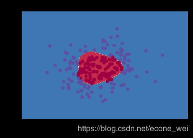
4 - 函数功能：可视化数据分类

def plot_decision_boundary(model, X, y):
    # 参数model的作用：对坐标值进行预测，（用训练好的模型对坐标预测，可以划分区域）
    # Set min and max values and give it some padding
    x_min, x_max = X[0, :].min() - 1, X[0, :].max() + 1
    y_min, y_max = X[1, :].min() - 1, X[1, :].max() + 1
    h = 0.01
    # Generate a grid of points with distance h between them
    xx, yy = np.meshgrid(np.arange(x_min, x_max, h), np.arange(y_min, y_max, h))
    Z = model(np.c_[xx.ravel(), yy.ravel()])
    Z = Z.reshape(xx.shape) 
    #  Z 的主要功能是对每个坐标都设置颜色变量
    # Plot the contour and training examples
    plt.contourf(xx, yy, Z, cmap=plt.cm.Spectral)
    plt.ylabel('x2')
    plt.xlabel('x1')
    plt.scatter(X[0, :], X[1, :], c=y, cmap=plt.cm.Spectral)
    

# Plot the decision boundary
plot_decision_boundary(lambda x: predict(parameters, x.T), X, Y.reshape(-1,))
plt.title("Decision Boundary for hidden layer unit " + str(4))

欢迎各位留言，一起探讨。