机器学习项目--加州房地产价格预测
本项目选取StatLib的加州房地产价格数据集,如下图:
1.问题总览
任务是利用加州普查数据,建立一个加州房价模型。这个数据包含每个街区组的人口、收入中位数、房价中位数等指标。
我们的模型要利用这个数据进行学习,然后根据其他指标,预测任何街区的房价中位数。
划定问题
商业目标是什么?设计的系统将如何被使用
模型的输出(一个区的房价中位数)会传给另一个机器学习系统,也有其他信号会传入后面的系统。这一整套系统可以确定某个区进行投资值不值。确定值不值得投资非常重要,它直接影响利润。
如果有,现在的解决方案效果如何?
现在街区的房价是靠专家手工估计的,专家队伍收集最新的关于一个区的信息(不包括房价中位数),他们使用复杂的规则进行估计。这种方法费钱费时间,而且估计结果不理想。
确定是哪种机器学习问题
这个问题是典型监督学习的问题,每个实例都有标签,即街区房价的中位数。
这个问题也是典型的回归问题,是一个多变量回归问题(人口、收入等),来预测一个值。
最后,这也是一个批量学习的问题,因为数据量完全可以放到内存中。
选择性能指标
回归问题的典型指标是均方根误差:
R M S E ( X , h ) = 1 m ∑ i = 1 m ( h ( x i ) − y i ) 2 RMSE(X,h)=\sqrt{\frac1m\sum_{i=1}^m(h(x^i)-y^i)^2} RMSE(X,h)=m1i=1∑m(h(xi)−yi)2
m:实例数量
x(i):实例i的特征向量
y(i):实例i的标签
h:系统预测函数,也称为假设
另外一种性能指标是平均绝对误差:
M A E ( X , h ) = 1 m ∑ i = 1 m ∣ h ( x i ) − y i ∣ MAE(X,h)=\frac1m\sum_{i=1}^m|h(x^i)-y^i| MAE(X,h)=m1i=1∑m∣h(xi)−yi∣
2.获取数据
数据源
下载数据
# 下载数据压缩包并解压
import os
import tarfile
import urllib.request

import ssl
ssl._create_default_https_context = ssl._create_unverified_context

DOWNLOAD_ROOT = "https://raw.githubusercontent.com/ageron/handson-ml/master/"
HOUSING_PATH = "datasets/housing"
HOUSING_URL = DOWNLOAD_ROOT + HOUSING_PATH + "/housing.tgz"


def fetch_housing_data(housing_url=HOUSING_URL):
    if not os.path.isdir(housing_url):
        os.makedirs(HOUSING_PATH)
    tgz_path = os.path.join(HOUSING_PATH, "housing.tgz")
    urllib.request.urlretrieve(housing_url, tgz_path)
    housing_tgz = tarfile.open(tgz_path)
    housing_tgz.extractall(path=HOUSING_PATH)
    housing_tgz.close()


fetch_housing_data()
查看数据
# 加载数据集
import pandas as pd
import os

HOUSING_PATH = "datasets/housing"

def load_housing_data(housing_path=HOUSING_PATH):
    csv_path = os.path.join(housing_path, "housing.csv")
    return pd.read_csv(csv_path)

raw_data = load_housing_data()
raw_data.head()
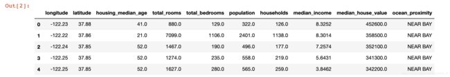
每行数据表示一个街区。共十个属性longitude, latitude, housing_median_age, total_rooms, total_bedrooms, population, households, median_income, median_house_value, ocean_proximity。
查看整体数据结构
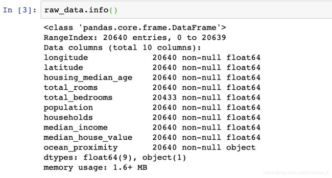
可以看到total_bedroom不是所有数据都有值(20433/20640),处理的时候需要小心。
ocean_proximity显然是个枚举值,可以通过下面的方法查询所有的枚举值。

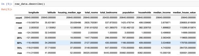
查看所有属性的基本信息
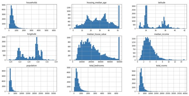
用matplotlib可视化数据
import matplotlib.pyplot as plt
raw_data.hist(bins=50, figsize=(20, 10))
plt.show()
创建测试集
随机从数据中抽取%20作为测试数据。
# 创建测试集,随机从数据中抽取%20作为测试集
import numpy as np

def split_train_test(data, test_ratio):
    # seed方法保证相同的种子每次随机生成的数组一致,即保证了测试集的一致
    np.random.seed(714)
    '''
    numpy.random中函数shuffle与permutation都是对原来的数组进行重新洗牌(即随机打乱原来的元素顺序);
    区别在于shuffle直接在原来的数组上进行操作,改变原来数组的顺序,无返回值。
    而permutation不直接在原来的数组上进行操作,而是返回一个新的打乱顺序的数组,并不改变原来的数组。
    当然,这里只是数组下标的打乱。
    '''
    shuffled_indices = np.random.permutation(len(data))
    test_set_size = int(len(data) * test_ratio)
    test_indices = shuffled_indices[:test_set_size]
    train_indices = shuffled_indices[test_set_size:]
    # iloc: 根据标签的所在位置,从0开始计数,选取列
    return data.iloc[train_indices], data.iloc[test_indices]

train_set, test_set = split_train_test(raw_data, 0.2)
print(len(train_set), "train +", len(test_set), "test")
# 16512 train + 4128 test
那么问题来了,如果源数据有更新,如何保证测试集不变?
一个通常的解决办法是使用每个实例的ID来判定这个实例是否应该放入测试集(假设每个实例都有唯一并且不变的ID)。例如,你可以计算出每个实例ID的哈希值,只保留其最后一个字节,如果该值小于等于 51(约为 256 的20%),就将其放入测试集。
import hashlib

def test_set_check(identifier, test_ratio, hash):
    return hash(np.int64(identifier)).digest()[-1] < 256 * test_ratio

def split_train_test_by_id(data, test_ratio, id_column, hash=hashlib.md5):
    ids = data[id_column]
    in_test_set = ids.apply(lambda id_: test_set_check(id_, test_ratio, hash))
    return data.loc[~in_test_set], data.loc[in_test_set]

#  添加一列index,从0开始
raw_data_with_id = raw_data.reset_index()
train_set, test_set = split_train_test_by_id(raw_data_with_id, 0.2, "index")

# 更好的办法是选择永远不会变的index:
# raw_data_with_id["index"] = raw_data["longitude"] * 1000 + housing["latitude"]
# 因为经纬度是永远不会变的

#hashlib基本用法:

#import hashlib
#md5 = hashlib.md5()
#md5.update('how to use md5 in python hashlib?')
#print(md5.hexdigest())
分层采样
目前为止的采样都是随机采样,在数据集非常大的时候没有问题,但如果数据集不大,就需要分层采样(stratified sampling),从每个分层取合适数量的实例,以保证测试集具有代表性。
import numpy as np
# 根据原始数据直方图中median_income的分布,新增一列income_cat,将数据映射到1-5之间
raw_data["income_cat"] = np.ceil(raw_data["median_income"] / 1.5) # ceil 向上取整
raw_data["income_cat"].where(raw_data["income_cat"] < 5, 5.0, inplace=True) # where(condition, other=NAN), 满足condition,则保留,不满足取other

raw_data["income_cat"].value_counts() / len(raw_data) # 查看不同收入分类的比例

from sklearn.model_selection import StratifiedShuffleSplit

split = StratifiedShuffleSplit(n_splits=1, test_size=0.2, random_state=42) # n_splites 将训练数据分成train/test对的组数
for train_index, test_index in split.split(raw_data, raw_data["income_cat"]): # split.split(X, y, groups=None) 根据y对X进行分割
    strat_train_set = raw_data.loc[train_index]
    strat_test_set = raw_data.loc[test_index]

# pandas中iloc和loc的区别:
#  iloc主要使用数字来索引数据,而不能使用字符型的标签来索引数据。而loc则刚好相反,只能使用字符型标签来索引数据,不能使用数字来索引数据

# 最后在数据中删除添加的income_cat列
for set in (strat_train_set, strat_test_set):
    set.drop(["income_cat"], axis=1, inplace=True)
# drop函数默认删除行,列需要加axis = 1, 它不改变原有的df中的数据,而是返回另一个dataframe来存放删除后的数据。
3.数据可视化,探索规律
创建数据副本
# 创建副本
housing = strat_train_set.copy()
可视化
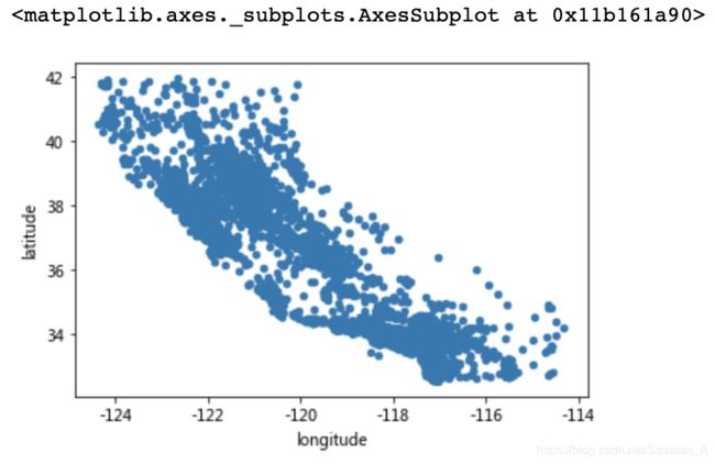
首先很直观的,看下经纬度的散点图
housing.plot(kind="scatter", x="longitude", y="latitude")
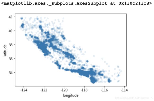
将alpha设为0.1可以看出地理位置信息的密度分布。
housing.plot(kind="scatter", x="longitude", y="latitude", alpha=0.1)
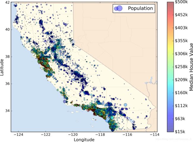
再加入人口和房价信息,每个圈的半径表示人口(population),圈的颜色表示房价(median_house_value)。
housing.plot(kind="scatter", x="longitude", y="latitude", alpha=0.4,
    s=housing["population"]/100, label="population",
    c="median_house_value", cmap=plt.get_cmap("jet"), colorbar=True)
plt.legend()
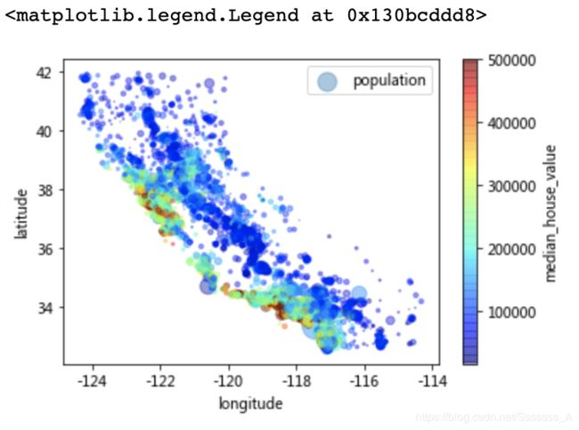
目测的规律:房价与人口密度密切相关,离大海的距离也是一个很有用的属性。
查找关联
from pandas.plotting import scatter_matrix
# 计算一下四个属性之间的关联性
attributes = ["median_house_value", "median_income", "total_rooms", "housing_median_age"]
scatter_matrix(housing[attributes], figsize=(12, 8))
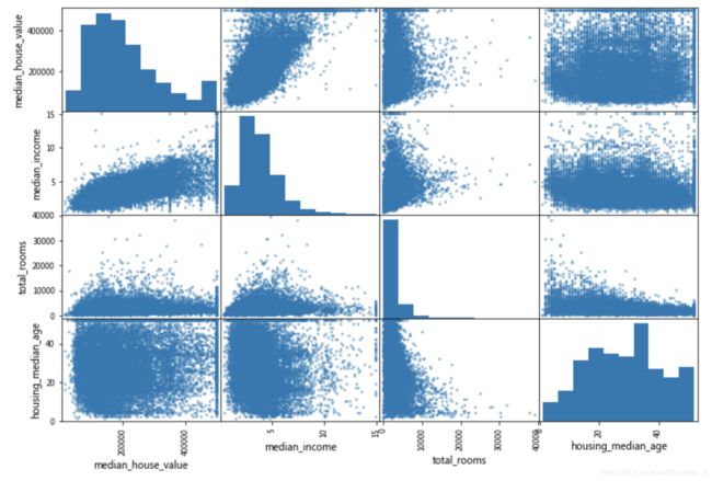
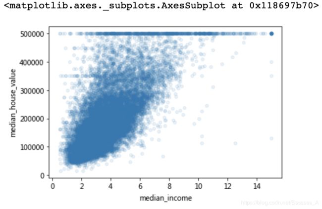
median_income与房价的相关性最大,把这个图单独拿出来。
housing.plot(kind="scatter", x="median_income",y="median_house_value", alpha=0.1)
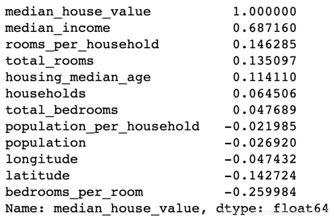
属性组合实验
给算法准备数据之前,你需要做的最后一件事是尝试多种属性组合。例如,如果你不知道某个街区有多少户,该街区的总房间数就没什么用。你真正需要的是每户有几个房间。相似的,总卧室数也不重要:你可能需要将其与房间数进行比较。每户的人口数也是一个有趣的属性组合。让我们来创建这些新的属性:
housing["rooms_per_household"] = housing["total_rooms"]/housing["households"]
housing["bedrooms_per_room"] = housing["total_bedrooms"]/housing["total_rooms"]
housing["population_per_household"]=housing["population"]/housing["households"]

corr_matrix = housing.corr()
corr_matrix["median_house_value"].sort_values(ascending=False)
# 新属性与房价的关联系数
小结
这一步的数据探索不必非常完备,此处的目的是有一个正确的开始,快速发现规律,以得到一个合理的原型。但是这是一个交互过程:一旦你得到了一个原型,并运行起来,你就可以分析它的输出,进而发现更多的规律,然后再回到数据探索这步。
4.准备用于机器学习算法的数据
先把属性和标签分开
housing = strat_train_set.drop("median_house_value", axis=1)
housing_labels = strat_train_set["median_house_value"].copy()
数据清洗
之前注意到有一些街区的total_bedrooms属性缺失。
Scikit-Learn 提供了一个方便的类来处理缺失值: Imputer
from sklearn.preprocessing import Imputer

imputer = Imputer(strategy="median")
# 因为只有数值属性才能算出中位数,我们需要创建一份不包括文本属性 ocean_proximity 的数据副本
housing_num = housing.drop("ocean_proximity", axis=1)
# imputer 计算出了每个属性的中位数,并将结果保存在了实例变量 statistics_ 中。
imputer.fit(housing_num)
# 使用这个“训练过的” imputer 来对训练集进行转换,将缺失值替换为中位数
X = imputer.transform(housing_num)
# 结果是一个包含转换后特征的普通的 Numpy 数组。将其放回到Pandas DataFrame 中。
housing_tr = pd.DataFrame(X, columns=housing_num.columns)
处理文本和类别属性Categorical Attributes
机器学习算法喜欢与数字打交道,所以将文本转换为数字
# 处理文本和类别属性 Categorical Attributes
# 数机器学习算法喜欢和数字打交道,所以将文本转换为数字
from sklearn.preprocessing import OrdinalEncoder

housing_cat = housing[['ocean_proximity']]
ordinal_encoder = OrdinalEncoder()
housing_cat_encoded = ordinal_encoder.fit_transform(housing_cat)
housing_cat_encoded[:10]

ordinal_encoder.categories_
# [array(['<1H OCEAN', 'INLAND', 'ISLAND', 'NEAR BAY', 'NEAR OCEAN'], dtype=object)]

# 这种做法的问题是,机器学习算法会认为两个临近的值比两个疏远的值要更相似,显然这样不对。
# 要解决这个问题,一个常见的方法是给每个分类创建一个二元属性:
#   当分类是 <1H OCEAN ,该属性为 1(否则为 0),当分类是 INLAND ,另一个属性等于 1(否则为 0),以此类推。
# 这称作独热编码(One-Hot Encoding),因为只有一个属性会等于 1(热),其余会是 0(冷)。

# OneHotEncoder ,用于将整数分类值转变为独热向量。注意 fit_transform() 用于 2D 数组,而 housing_cat_encoded 是一个 1D 数组,所以需要将其变形
from sklearn.preprocessing import OneHotEncoder

encoder = OneHotEncoder()
housing_cat_1hot = encoder.fit_transform(housing_cat_encoded.reshape(-1,1))
housing_cat_1hot # 输出是系数矩阵
#<16512x5 sparse matrix of type ''
#   with 16512 stored elements in Compressed Sparse Row format>

housing_cat_1hot.toarray() # 转换成密集矩阵,或者在初始化的时候 cat_encoder = OneHotEncoder(sparse=False)
array([[1., 0., 0., 0., 0.],
       [1., 0., 0., 0., 0.],
       [0., 0., 0., 0., 1.],
       ...,
       [0., 1., 0., 0., 0.],
       [1., 0., 0., 0., 0.],
       [0., 0., 0., 1., 0.]])
自定义转换器
尽管 Scikit-Learn 提供了许多有用的转换器,你还是需要自己动手写转换器执行任务,比如自定义的清理操作,或属性组合。你需要让自制的转换器与 Scikit-Learn 组件(比如流水线)无缝衔接工作,因为 Scikit-Learn 是依赖鸭子类型的(而不是继承),你所需要做的是创建一个类并执行三个方法: fit() (返回 self ), transform() ,和 fit_transform() 。通过添加 TransformerMixin 作为基类,可以很容易地得到最后一个。另外,如果你添加 BaseEstimator 作为基类(且构造器中避免使用 *args 和 **kargs ),你就能得到两个额外的方法( get_params() 和 set_params() ),二者可以方便地进行超参数自动微调。例如,一个小转换器类添加了上面讨论的属性:
# 自定义转换器
from sklearn.base import BaseEstimator, TransformerMixin

# column index
rooms_ix, bedrooms_ix, population_ix, household_ix = 3, 4, 5, 6

class CombinedAttributesAdder(BaseEstimator, TransformerMixin):
    def __init__(self, add_bedrooms_per_room = True): # no *args or **kargs
        self.add_bedrooms_per_room = add_bedrooms_per_room
    def fit(self, X, y=None):
        return self  # nothing else to do
    def transform(self, X, y=None):
        rooms_per_household = X[:, rooms_ix] / X[:, household_ix]
        population_per_household = X[:, population_ix] / X[:, household_ix]
        if self.add_bedrooms_per_room:
            bedrooms_per_room = X[:, bedrooms_ix] / X[:, rooms_ix]
            return np.c_[X, rooms_per_household, population_per_household,
                         bedrooms_per_room]
        else:
            return np.c_[X, rooms_per_household, population_per_household]

attr_adder = CombinedAttributesAdder(add_bedrooms_per_room=False)
housing_extra_attribs = attr_adder.transform(housing.values)
特征缩放
线性归一化
通过减去最小值,然后再除以最大值与最小值的差值,来进行归一化。Scikit-Learn 提供了一个转换器 MinMaxScaler 来实现这个功能。它有一个超参数 feature_range ,可以让你改变范围,如果不希望范围是 0 到 1。
标准化
首先减去平均值(所以标准化值的平均值总是 0),然后除以方差,使得到的分布具有单位方差。标准化受到异常值的影响很小。Scikit-Learn 提供了一个转换器 StandardScaler 来进行标准化。
转换流水线
数据处理过程存在许多数据转换步骤,需要按一定的顺序执行。幸运的是,Scikit-Learn 提供了类 Pipeline ,来进行这一系列的转换。下面是一个数值属性的小流水线:
from sklearn.pipeline import Pipeline
from sklearn.preprocessing import StandardScaler
from sklearn.preprocessing import Imputer
from sklearn.compose import ColumnTransformer

# 构造器需要一个定义步骤顺序的名字/估计器对的列表。除了最后一个估计器,其余都要是转换器(即,它们都要有 fit_transform() 方法)。
# 当你调用流水线的 fit() 方法,就会对所有转换器顺序调用 fit_transform() 方法,将每次调用的输出作为参数传递给下一个调用,一直到最后一个估计器,它只执行 fit() 方法。

num_attribs = list(housing_num)
cat_attribs = ["ocean_proximity"]

num_pipeline = Pipeline([
    ('imputer', Imputer(strategy="median")),
    ('attribs_adder', CombinedAttributesAdder()),
    ('std_scaler', StandardScaler()),
    ])

full_pipeline = ColumnTransformer([
        ("num", num_pipeline, num_attribs),
        ("cat", OneHotEncoder(), cat_attribs),
    ])

housing_prepared = full_pipeline.fit_transform(housing)

housing_prepared.shape
# (16512, 16)
5.选择模型并进行训练
先训练一个线性回归模型
from sklearn.linear_model import LinearRegression

lin_reg = LinearRegression()
lin_reg.fit(housing_prepared, housing_labels)
计算RMSE
from sklearn.metrics import mean_squared_error

housing_predictions = lin_reg.predict(housing_prepared)
lin_mse = mean_squared_error(housing_labels, housing_predictions)
lin_rmse = np.sqrt(lin_mse)
lin_rmse
# 输出结果为68628.19819848922
因此预测误差68628不能让人满意。这是一个模型欠拟合训练数据的例子。当这种情况发生时,意味着特征没有提供足够多的信息来做出一个好的预测,或者模型并不强大。
换一个决策树模型
from sklearn.tree import DecisionTreeRegressor

tree_reg = DecisionTreeRegressor()
tree_reg.fit(housing_prepared, housing_labels)

housing_predictions = tree_reg.predict(housing_prepared)
tree_mse = mean_squared_error(housing_labels, housing_predictions)
tree_rmse = np.sqrt(tree_mse)
tree_rmse
# 最后输出0.0 大概率过拟合了
交叉验证
# 随机地将训练集分成十个不同的子集,然后训练评估决策树模型 10 次,每次选一个不用的折来做评估,
# 用其它 9 个来做训练。结果是一个包含10 个评分的数组。

from sklearn.model_selection import cross_val_score

scores = cross_val_score(tree_reg, housing_prepared, housing_labels,
                         scoring="neg_mean_squared_error", cv=10)
tree_rmse_scores = np.sqrt(-scores)
tree_rmse_scores
# array([68274.11882883, 66569.14495813, 72556.31339841, 68235.85607159,
#       70706.44616166, 73298.7766776 , 70404.07783425, 71858.98228216,
#       77435.9399421 , 71396.89318558])
"""
Scikit-Learn 交叉验证功能期望的是效用函数(越大越好)
"""

def display_scores(scores):
    print("Scores:", scores)
    print("Mean:", scores.mean())
    print("Standard deviation:", scores.std())

display_scores(tree_rmse_scores)
输出结果:
Scores: [68883.6930069  66065.30851291 69754.34679347 69129.20768633
 71165.52382571 73746.5102225  71513.85226866 72387.84216761
 78097.08832454 70375.37813418]
Mean: 71111.87509428067
Standard deviation: 3070.4392604867644
再换一个随机森林
from sklearn.ensemble import RandomForestRegressor

forest_reg = RandomForestRegressor(random_state=42)
forest_reg.fit(housing_prepared, housing_labels)
housing_predictions = forest_reg.predict(housing_prepared)
forest_mse = mean_squared_error(housing_labels, housing_predictions)
forest_rmse = np.sqrt(forest_mse)
forest_rmse
# 21933.31414779769
forest_scores = cross_val_score(forest_reg, housing_prepared, housing_labels,
                                scoring="neg_mean_squared_error", cv=10)
forest_rmse_scores = np.sqrt(-forest_scores)
display_scores(forest_rmse_scores)
输出结果:
Scores: [51646.44545909 48940.60114882 53050.86323649 54408.98730149
 50922.14870785 56482.50703987 51864.52025526 49760.85037653
 55434.21627933 53326.10093303]
Mean: 52583.72407377466
Standard deviation: 2298.353351147122
保存模型
from sklearn.externals import joblib

joblib.dump(forest_reg, "my_model.pkl")
# 然后
my_model_loaded = joblib.load("my_model.pkl")
6.模型微调
网格搜索Grid Search
下面的代码搜索了 RandomForestRegressor 超参数值的最佳组合:
from sklearn.model_selection import GridSearchCV

param_grid = [
    # try 12 (3×4) combinations of hyperparameters
    {'n_estimators': [3, 10, 30], 'max_features': [2, 4, 6, 8]},
    # then try 6 (2×3) combinations with bootstrap set as False
    {'bootstrap': [False], 'n_estimators': [3, 10], 'max_features': [2, 3, 4]},
  ]

forest_reg = RandomForestRegressor(random_state=42)
# train across 5 folds, that's a total of (12+6)*5=90 rounds of training
grid_search = GridSearchCV(forest_reg, param_grid, cv=5,
                           scoring='neg_mean_squared_error', return_train_score=True)
grid_search.fit(housing_prepared, housing_labels)
grid_search.best_params_
# {'max_features': 8, 'n_estimators': 30}
# 因为 30 是 n_estimators 的最大值,你也应该估计更高的值,因为评估的分数可能会随 n_estimators 的增大而持续提升。
输出:
{'max_features': 8, 'n_estimators': 30}
随机搜索
from sklearn.model_selection import RandomizedSearchCV
from scipy.stats import randint

param_distribs = {
        'n_estimators': randint(low=1, high=200),
        'max_features': randint(low=1, high=8),
    }

forest_reg = RandomForestRegressor(random_state=42)
rnd_search = RandomizedSearchCV(forest_reg, param_distributions=param_distribs,
                                n_iter=10, cv=5, scoring='neg_mean_squared_error', random_state=42)
rnd_search.fit(housing_prepared, housing_labels)
输出:
RandomizedSearchCV(cv=5, error_score='raise-deprecating',
                   estimator=RandomForestRegressor(bootstrap=True,
                                                   criterion='mse',
                                                   max_depth=None,
                                                   max_features='auto',
                                                   max_leaf_nodes=None,
                                                   min_impurity_decrease=0.0,
                                                   min_impurity_split=None,
                                                   min_samples_leaf=1,
                                                   min_samples_split=2,
                                                   min_weight_fraction_leaf=0.0,
                                                   n_estimators='warn',
                                                   n_jobs=None, oob_score=False,
                                                   random_sta...
                                                   warm_start=False),
                   iid='warn', n_iter=10, n_jobs=None,
                   param_distributions={'max_features': <scipy.stats._distn_infrastructure.rv_frozen object at 0x135681588>,
                                        'n_estimators': <scipy.stats._distn_infrastructure.rv_frozen object at 0x135681f28>},
                   pre_dispatch='2*n_jobs', random_state=42, refit=True,
                   return_train_score=False, scoring='neg_mean_squared_error',
                   verbose=0)
分析最佳模型和它们的误差
用测试集评估系统
# 用测试集评估系统
final_model = grid_search.best_estimator_
X_test = strat_test_set.drop("median_house_value", axis=1)
y_test = strat_test_set["median_house_value"].copy()
X_test_prepared = full_pipeline.transform(X_test)
final_predictions = final_model.predict(X_test_prepared)
final_mse = mean_squared_error(y_test, final_predictions)
final_rmse = np.sqrt(final_mse)
# 47730.22690385927

final_rmse
47730.22690385927