TensorFlow入门之CIFAR-10图像识别模型实战教程

---

下载TensorFlow Models库

下载Tensorflow Models库，以便使用其中提供的CIFAR-10数据的类。
注意：在git中进行操作，没有安装git的先安装git。

# 下载Tensorflow Models库，可能需要较长时间，耐心等待，切忌中途结束否则重新下载比较麻烦
git clone https://github.com/tensorflow/models.git
# 下载好Tensorflow Models库后进cifar10所在位置
cd models/tutorials/image/cifar10

TensorFlow官方示例的CIFAR-10代码文件

文件	用途
cifar10.py	建立CIFAR-10预测模型
cifar10_input.py	在TensorFlow中读入CIFAR-10训练图片
cifar10_input_test.py	cifar10_input的测试用例文件
cifar10_train.py	使用单个GPU或CPU训练模型
cifar10_train_multi_gpu.py	使用多个GPU训练模型
cifar10_eval.py	在测试集上测试模型的性能

---

CIFAR-10数据集

CIFAR-10数据集介绍

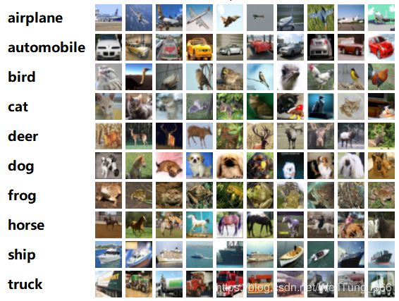
CIFAR-10是一个用于识别普适物体的小型数据据，它一共包含10个类别的RGB彩色图片：飞机（ airplane ）、汽车（ automobile ）、鸟类（ bird ）、猫（ cat ）、鹿（ deer ）、狗（ dog ）、蛙类（ frog ）、马（ horse ）、船（ ship ）和卡车（ truck ）。图片的尺寸为 32×32 ，数据集中一共有 50000 张训练图片和 10000 张测试图片。 如下图示：

下载CIFAR-10数据

CIFAR-10数据集可以自己下载也可以直接从Tensorflow Models库中自动下载。

下载地址：http://www.cs.toronto.edu/~kriz/cifar.html

点击进入下载地址，选择python版本进行下载。

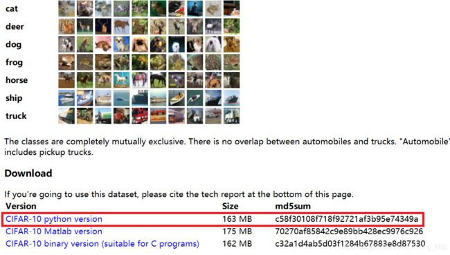
下载完成后得到一个cifar-1-pythoin.tar.gz解压包

将cifar-1-pythoin.tar.gz解压包解压得到cifar-10-batches-py文件夹

数据文件名及用途

文件名	文件用途
batches.meta.txt	文本文件，存储了每个类别的英文名称。可以用记事本或其他文本文件阅读器打开浏览
data_batch_1.bin、… 、data_batch_5.bin	这 5 个文件是 CIFAR-10 数据集中的训练数据，每个文件以二进制格式存储了 10000 张 32×32的彩色图像和这些图像对应的类别标签，一共 50000 张训练图像
test_batch.bin	这个文件存储的是测试图像和测试图像的标签，一共10000 张
readme.html	数据集介绍文件

---

开始训练模型

导入包和定义参数

导入常用库并载入TensorFlow Models中自动下载、读取CIFAR-10数据的类

import tensorflow as tf
import numpy as np
import time
import cifar10,cifar10_input

定义batch_size、训练轮数max_steps和下载CIFAR-10数据的默认路径

# 最大迭代轮数
max_steps = 3000 
# 批大小
batch_size = 128   
# 数据所在路径
data_dir = '/tmp/cifar10_data/cifar-10-batches-bin'  

定义初始化weight的函数

使用tf.truncated_normal截断的正态分布来初始化权重，再给weight增加一个L2的loss，相当于给L2做了一个正则化。用wl控制L2loss的大小。使用tf.nn.l2_loss函数计算weight的L2loss，再使用tf.multipl让L2乘wl得到最终的weight loss。最后使用tf.add_to_collection把weight loss统一存储到一个名为“losses”的collection中，在后面计算神经网络总体loss时被用上。

def _variable_with_weight_loss(shape, stddev, wd):
  var = tf.Variable(tf.truncated_normal(shape, stddev=stddev))
  if wd is not None:
    weight_decay = tf.multiply(tf.nn.l2_loss(var), wd, name='weight_loss')
    tf.add_to_collection('losses', weight_decay)
  return var

tf.nn.l2_loss(t, name=None )：用于优化的目标函数中的正则项，防止参数太多复杂容易过拟合。
tf.add_to_collection()：向当前计算图中添加张量集合

下载数据集并解压展开到默认位置

cifar10.maybe_download_and_extract()

数据增强和输入

使用cifar10_input类中的distorted_inputs函数产生训练和测试需要使用的数据，包括特征及其对应的label。（已经对数据进行数据增强）

# 训练数据
images_train, labels_train = cifar10_input.distorted_inputs(data_dir=data_dir, batch_size=batch_size)
# 测试数据
images_test, labels_test = cifar10_input.inputs(eval_data=True, data_dir=data_dir, batch_size=batch_size)

创建输入数据的placeholder，包括特征和label

# 尺寸为24×24，颜色通道设为3，代表图片是彩色有RGB三条通道
image_holder = tf.placeholder(tf.float32, [batch_size, 24, 24, 3])
label_holder = tf.placeholder(tf.int32, [batch_size])

定义神经网络

卷积层一

# 卷积核大小为5×5，3个颜色通道，54个卷经核，weight初始化函数的标准差为0.05
weight1 = _variable_with_weight_loss(shape=[5, 5, 3, 64],stddev=5e-2,wd=0.0)

# 卷积操作，步长为1，padding设为SAME
kernel1 = tf.nn.conv2d(image_holder, weight1, [1, 1, 1, 1], padding='SAME')

# bias全部初始化为0
bias1 = tf.Variable(tf.constant(0.0, shape=[64]))

# 使用ReLu激活函数进行非线性化
conv1 = tf.nn.relu(tf.nn.bias_add(kernel1, bias1))

# 使用一个尺寸为3×3，步长为2的×2的最大池化层（最大池化的尺寸和步长不一样可以增加数据的丰富性）
pool1 = tf.nn.max_pool(conv1, ksize=[1, 3, 3, 1], strides=[1, 2, 2, 1],padding='SAME')

# 使用tf.nn.lrn函数对结果进行处理（增强模型的泛化能力）
norm1 = tf.nn.lrn(pool1, 4, bias=1.0, alpha=0.001 / 9.0, beta=0.75)

卷积层二

weight2 = _variable_with_weight_loss([5, 5, 64, 64], stddev=5e-2, wd=0.0)
kernel2 = tf.nn.conv2d(norm1, weight2, strides=[1, 1, 1, 1], padding='SAME')
# bias初始为0.1，而不是0
bias2 = tf.Variable(tf.constant(0.1, shape=[64]))
conv2 = tf.nn.relu(tf.nn.bias_add(kernel2, bias2))
# 调换了LRN和池化的顺序
norm2 = tf.nn.lrn(conv2, 4, bias=1.0, alpha=0.001 / 9.0, beta=0.75)
pool2 = tf.nn.max_pool(norm2, ksize=[1, 3, 3, 1],strides=[1, 2, 2, 1], padding='SAME')

全连接层三

# 使用 tf.reshape将样本都变成一维
reshape = tf.reshape(pool2, [batch_size, -1]) 
# 获取数据扁平化后的长度
dim = reshape.get_shape()[1].value  
# 使用_variable_with_weight_loss函数对全连接层的weight初始化
weight3 = _variable_with_weight_loss([dim, 384], stddev=0.04, wd=0.004)
bias3 = tf.Variable(tf.constant(0.1, shape=[384]))
local3 = tf.nn.relu(tf.matmul(reshape, weight3) + bias3)

全连接层四

weight4 = _variable_with_weight_loss([384, 192], stddev=0.04, wd=0.004)
bias4 = tf.Variable(tf.constant(0.1, shape=[192]))
local4 = tf.nn.relu(tf.matmul(local3, weight4) + bias4)

全连接层五

weight5 = _variable_with_weight_loss([192, 10],stddev=1/192.0, wd=0.0)
bias5 = tf.Variable(tf.constant(0.0, shape=[10]))
logits = tf.add(tf.matmul(local4, weight5), bias5)

卷积神经网络及结构表

Layer名称	描 述
conv1	卷积层和ReLu激活函数
pool1	最大池化
norm1	LRN
conv2	卷积层和ReLu激活函数
norm2	LRN
pool2	最大池化
local3	全连接层和ReLu激活函数
local4	全连接层和ReLu激活函数
logits	模型Inference的输出结果

计算损失函数loss

def loss(logits, labels):
  labels = tf.cast(labels, tf.int64)
  cross_entropy = tf.nn.sparse_softmax_cross_entropy_with_logits(labels=labels, logits=logits, name='cross_entropy_per_example')
  cross_entropy_mean = tf.reduce_mean(cross_entropy, name='cross_entropy')
  tf.add_to_collection('losses', cross_entropy_mean)
  return tf.add_n(tf.get_collection('losses'), name='total_loss')

# 将logits节点和label_placeholder传入loss函数获得最终的loss
loss = loss(logits, label_holder)

# 优化器使用Adam Optimizer，学习率设为1e-3
train_op = tf.train.AdamOptimizer(1e-3).minimize(loss) 

# 使用tf.nn.in_top_k函数求输出top k的准确率，默认使用top 1，也就是输出分数最高那一类的准确率
top_k_op = tf.nn.in_top_k(logits, label_holder, 1)

创建Sessionc，初始化参数

使用tf.InteractiveSession创建默认Seesion，接着初始化模型的全部参数

sess = tf.InteractiveSession()
tf.global_variables_initializer().run()

启动图片数据增强的线程队列

tf.train.start_queue_runners()

迭代训练

for step in range(max_steps):
    start_time = time.time()
    # 获取训练数据
    image_batch, label_batch = sess.run([images_train, labels_train]) 
     # 计算每次迭代需要的时间
    _, loss_value = sess.run([train_op, loss],feed_dict={image_holder: image_batch,label_holder: label_batch})
    duration = time.time() - start_time
    if step % 10 == 0:
        examples_per_sec = batch_size / duration 
        sec_per_batch = float(duration) 
        format_str = ('step %d, loss=%.2f (%.1f examples/sec; %.3f sec/batch)')
        print(format_str % (step, loss_value, examples_per_sec, sec_per_batch))

在测试集上测评准确率

num_examples = 10000
import math

num_iter = int(math.ceil(num_examples / batch_size))
true_count = 0
total_sample_count = num_iter * batch_size
step = 0
while step < num_iter:
    image_batch, label_batch = sess.run([images_test, labels_test])
    predictions = sess.run([top_k_op],feed_dict={image_holder: image_batch,label_holder: label_batch})
    true_count += np.sum(predictions)
    step += 1

precision = true_count / total_sample_count
print('precision @ 1 =%.3f' % precision)

最终训练的准确率约为：73%

---

全部代码

import tensorflow as tf
import numpy as np
import time
import cifar10,cifar10_input

max_steps = 3000  
batch_size = 128    
data_dir = '/tmp/cifar10_data/cifar-10-batches-bin' 



def _variable_with_weight_loss(shape, stddev, wd):
  var = tf.Variable(tf.truncated_normal(shape, stddev=stddev))
  if wd is not None:
    weight_decay = tf.multiply(tf.nn.l2_loss(var), wd, name='weight_loss')
    tf.add_to_collection('losses', weight_decay)
  return var

cifar10.maybe_download_and_extract()


images_train, labels_train = cifar10_input.distorted_inputs(data_dir=data_dir, batch_size=batch_size)
images_test, labels_test = cifar10_input.inputs(eval_data=True, data_dir=data_dir, batch_size=batch_size)

image_holder = tf.placeholder(tf.float32, [batch_size, 24, 24, 3])
label_holder = tf.placeholder(tf.int32, [batch_size])

weight1 = _variable_with_weight_loss(shape=[5, 5, 3, 64],stddev=5e-2,wd=0.0)
kernel1 = tf.nn.conv2d(image_holder, weight1, [1, 1, 1, 1], padding='SAME')
bias1 = tf.Variable(tf.constant(0.0, shape=[64]))
conv1 = tf.nn.relu(tf.nn.bias_add(kernel1, bias1))
pool1 = tf.nn.max_pool(conv1, ksize=[1, 3, 3, 1], strides=[1, 2, 2, 1],padding='SAME')
norm1 = tf.nn.lrn(pool1, 4, bias=1.0, alpha=0.001 / 9.0, beta=0.75)

weight2 = _variable_with_weight_loss([5, 5, 64, 64], stddev=5e-2, wd=0.0)
kernel2 = tf.nn.conv2d(norm1, weight2, strides=[1, 1, 1, 1], padding='SAME')
bias2 = tf.Variable(tf.constant(0.1, shape=[64]))
conv2 = tf.nn.relu(tf.nn.bias_add(kernel2, bias2))
norm2 = tf.nn.lrn(conv2, 4, bias=1.0, alpha=0.001 / 9.0, beta=0.75)
pool2 = tf.nn.max_pool(norm2, ksize=[1, 3, 3, 1],strides=[1, 2, 2, 1], padding='SAME')

reshape = tf.reshape(pool2, [batch_size, -1]) 
dim = reshape.get_shape()[1].value  
weight3 = _variable_with_weight_loss([dim, 384], stddev=0.04, wd=0.004)
bias3 = tf.Variable(tf.constant(0.1, shape=[384]))
local3 = tf.nn.relu(tf.matmul(reshape, weight3) + bias3)

weight4 = _variable_with_weight_loss([384, 192], stddev=0.04, wd=0.004)
bias4 = tf.Variable(tf.constant(0.1, shape=[192]))
local4 = tf.nn.relu(tf.matmul(local3, weight4) + bias4)

weight5 = _variable_with_weight_loss([192, 10],stddev=1/192.0, wd=0.0)
bias5 = tf.Variable(tf.constant(0.0, shape=[10]))
logits = tf.add(tf.matmul(local4, weight5), bias5)


def loss(logits, labels):
  labels = tf.cast(labels, tf.int64)
  cross_entropy = tf.nn.sparse_softmax_cross_entropy_with_logits(labels=labels, logits=logits, name='cross_entropy_per_example')
  cross_entropy_mean = tf.reduce_mean(cross_entropy, name='cross_entropy')
  tf.add_to_collection('losses', cross_entropy_mean)
  return tf.add_n(tf.get_collection('losses'), name='total_loss')

loss = loss(logits, label_holder)
train_op = tf.train.AdamOptimizer(1e-3).minimize(loss) 
top_k_op = tf.nn.in_top_k(logits, label_holder, 1)


sess = tf.InteractiveSession()
tf.global_variables_initializer().run()
tf.train.start_queue_runners()


for step in range(max_steps):
    start_time = time.time()
    image_batch, label_batch = sess.run([images_train, labels_train]) 
    _, loss_value = sess.run([train_op, loss],feed_dict={image_holder: image_batch,label_holder: label_batch})
    duration = time.time() - start_time
    if step % 10 == 0:
        examples_per_sec = batch_size / duration 
        sec_per_batch = float(duration) 
        format_str = ('step %d, loss=%.2f (%.1f examples/sec; %.3f sec/batch)')
        print(format_str % (step, loss_value, examples_per_sec, sec_per_batch))

num_examples = 10000
import math

num_iter = int(math.ceil(num_examples / batch_size))
true_count = 0
total_sample_count = num_iter * batch_size
step = 0
while step < num_iter:
    image_batch, label_batch = sess.run([images_test, labels_test])
    predictions = sess.run([top_k_op],feed_dict={image_holder: image_batch,label_holder: label_batch})
    true_count += np.sum(predictions)
    step += 1

precision = true_count / total_sample_count
print('precision @ 1 =%.3f' % precision)

---

项目代码

GitHub地址：https://github.com/WellTung666/Tensorflow/tree/master/CIFAR-10

---

参考资料

TensorFlow实战