Tensorflow 模型量化 (Quantizing deep convolutional networks for efficient inference: A whitepaper 译文)
最近Tensorflow官方发布了一份《Quantizing deep convolutional networks for efficient inference》白皮书,共36页,讲解了基于Tensorflow的模型量化的有关知识。由于最近也在学习模型量化这部分工作,所以计划对这份文档翻译一下,同时share给大家。由于工作时间所限,我尽量每天翻译一些,如果有误解的地方,也请大家批评指正。
2018.07.30
如需转载,请注明出处: https://blog.csdn.net/guvcolie/article/details/81286349
1 Introduction
Deep networks are increasingly used for applications at the edge. Devices at the edge typically have lower compute capabilities and are constrained in memory and power consumption. It is also necessary to reduce the amount of communication to the cloud for transferring models to the device to save on power and reduce network connectivity requirements. Therefore, there is a pressing need for techniques to optimize models for reduced model size, faster inference and lower power consumption.
深度神经网络已经逐渐地应用在周边应用中。在周边应用中的设备一般只有比较低的计算能力,而且也会受限于内存和电量消耗。也有必要降低将模型传输给设备的通信量及降低网络连接需求。因此,将模型量化使其模型尺寸更小、推断更快、耗电更低是非常有必要的。
There is extensive research on this topic with several approaches being considered:One approach is to build efficient models from the ground up [1],[2] and [3]. Another technique is to reduce the model size by applying quantization, pruning and compression techniques [4], [5] and [6]. Faster inference has been achieved by having efficient kernels for computation in reduced precision like GEMMLOWP [7], Intel MKL-DNN[8] , ARM CMSIS [9], Qualcomm SNPE [10], Nvidia TensorRT [11] and custom hardware for fast inference [12], [13] and [14].
对于这个主题,已经有广泛的研究可供参考:一种方法是从头构建一个高效的模型[1][2][3]。另一种技术是通过量化、裁剪和压缩来降低模型尺寸[4][5][6]。更快的推断可以通过在降低精度的前提下使用高效计算平台而达到,其中包括GEMMLOWP [7], Intel MKL-DNN[8] , ARM CMSIS [9], Qualcomm SNPE [10], Nvidia TensorRT [11] 以及用于快速推断的定制硬件 [12], [13] and [14].
One of the simpler ways to reduce complexity of any model is to reduce the precision requirements for the weights and activations. This approach has many advantages:
降低任何模型的复杂度的一种很简单的方法是降低权重和激活输出的精度要求。这种方法有很多优点:
- It is broadly applicable across a range of models and use cases. One does not need to develop a new model architecture for improved speed. In many cases, one can start with an existing floating point model and quickly quantize it to obtain a fixed point quantized model with almost no accuracy loss, without needing to retrain the model. Multiple hardware platforms and libraries support fast inference with quantized weights and activations, so there is no need to wait for new hardware development.
- 它适用于绝大多数模型和使用场景。我们不需要为了提高速度去开发一个信息模型结构。在许多情况下,我们根本不需要重新训练模型,只需要使用已有的浮点模型,然后就可以很快将其量化为定点型模型,而且几乎不会有精度损失。现在许多硬件平台和库都支持利用量化的权重和激活输出来进行快速推断,因此没必要等待新硬件的开发。
- Smaller Model footprint: With 8-bit quantization, one can reduce the model size a factor of 4, with negligible accuracy loss. This can be done without needing any data as only the weights are quantized. This also leads to faster download times for model updates.
- 更小的模型尺寸:使用8bit量化,我们可以将模型的尺寸降低4倍,而精度损失很小。这种方法不需要任何数据,只需要将权重量化就可实现。这对于模型更新来讲,也可以减少模型下载时间。
- Less working memory and cache for activations: Intermediate computations are typically stored in cache for reuse by later layers of a deep network and reducing the precision at which this data is stored leads to less working memory needed. Having lower precision weights and activations allows for better cache reuse.
- 更少的内存和缓存用于激活输出:中间计算结果为了网络的后续层重用,一般会缓存在cache中,而且降低精度这块数据就会占用更少的内存。既,更低精度的权重和激活输出有利于缓存更好地重用。
- Faster computation: Most processors allow for faster processing of 8-bit data.
- 更快地计算:大多数处理器支持8bit数据的更快处理功能。
- Lower Power: Moving 8-bit data is 4 times more efficient than moving 32-bit floating point data. In many deep architectures, memory access can dominate power consumption [2]. Therefore reduction in amount of data movement can have a significant impact on the power consumption.
- 低功耗:移动8bit定点型数据与移动32bit浮点型数据相比,在效率上前者比后者高4倍。对于许多深度网络结构,内存的使用量一定程度上正比于功耗[2]。因此减少数据移动量对降低功耗有非常重大的影响。
All the factors above translate into faster inference, with a typical speedup of 2-3x due to the reduced precision for both memory accesses and computations. Further improvements in speed and power consumption are possible with processors and hardware accelerators optimized for low precision vector arithmetic.
以上因素都可以使推断更快,由于降低数据精度而使内存占用和计算更少,一般会提速2-3倍。如果处理器或硬件加速器对低精度向量计算做过优化的话,速度和功耗有可能会进一步提升。
2 Quantizer Design (量化设计)
In this section, we review different design choices for uniform quantization.
在本节,我们回顾一下不同的量化设计方案。
2.1 Uniform Affine Quantizer
Consider a floating point variable with range (x min , x max ) that needs to be quantized to the range (0, N levels − 1) where N levels = 256 for 8-bits of precision. We derive two parameters: Scale (∆) and Zero-point(z) which map the floating point values to integers (See [15]). The scale specifies the step size of the quantizer and floating point zero maps to zero-point [4]. Zero-point is an integer, ensuring that zero is quantized with no error. This is important to ensure that common operations like zero padding do not cause quantization error. For one sided distributions, therefore, the range (x min , x max ) is relaxed to include zero. For example, a floating point variable with the range (2.1,3.5) will be relaxed to the range (0,3.5) and then quantized. Note that this can cause a loss of precision in the case of extreme one-sided distributions.
假设有一个浮点型变量,它的取值范围为(Xmin, Xmax),现在我们要把它量化到(0, N levels - 1)取值范围,其中对于8bit精度来讲N levels = 256。我们使用2个参数将浮点型值映射为整型值,尺度(∆)和零点(z)。尺度指定了量化的步长,浮点型0映射到零点。零点是一个整型数,确保0没有量化误差。对于像0 padding这种常用运算符不要产生量化误差是很重要的。对于单边分布,范围(Xmin,Xmax)需要进一步放宽去包含0点。例如,范围为(2.1, 3.5)的浮点型变量将会放宽为(0, 3.5),然后再量化。注意,这种方式对于极端的单边分布会产生精度损失。
Once the scale and zero-point are defined, quantization proceeds as follows:
一旦尺度和零点定义好了,量化过程如下:
The de-quantization operation is:
逆量化过程如下:
While the uniform affine quantizer allows for storing weights and activations at 8-bits of precision, there is an additional cost due to the zero-point. Consider a 2D convolution between a weight and an activation:
虽然“均匀映射量化”允许采用8bit精度来存储权重和激活输出,但因为零点,也会有一个额外的开销。考虑权重和激活输出之间的一个2D卷积:
A naive implementation of convolution, by performing the addition of zero-point prior to the convolution, leads to a 2x to 4x reduction in the throughput due to wider (16/32-bit) operands. One can do better by using the equation above and noting that the last term is a constant and each of the other terms requires N multiplies, which is 3x more operations than the 8-bit dot product. This can be further improved by noting that the weights are constant at inference and by noting that the sum over activations is identical for all convolutional kernels of the same size. However, this requires optimizing convolution kernels. For an indepth discussion, please see [16].
在卷积上加上一个零点先验的这种直接的卷积实现,会因为更宽操作数(16/32bit)的缘故,会导致吞吐量下降2到4倍。我们利用上面的公式,并注意到最后一项(原文中公式6部分)是一个常数而且其余项的每一项需要做N次相乘(这会比8bit点乘多出3倍计算量)这样的事实,可以进一步优化,因为在预测阶段权重都是常量了,而且对于一样尺寸的卷积核来讲计算得到的激活输出是一致的。但这需要优化卷积核。深入讨论请详见[16]。
2.2 Uniform symmetric quantizer
A simplified version of the affine quantizer is the symmetric quantizer, which restricts zero-point to 0. With the symmetric quantizer, the conversion operations simplify to:
映射量化的一个简化版本是symmetric quantizer“对称量化”,这种方法将零点约束到0位置。在对称量化方法中,转换操作可以简化为:
For faster SIMD implementation, we further restrict the ranges of the weights. In this case, the clamping is modified to:
对于更快的SIMD(SingleInstruction Multiple Data 单指令流多数据流)实现,我们要进一步约束权重的范围。这时,钳位运算可以简化为:
Please see [4], Appendix B for more details.
想了解更多细节,请详见[4]以及Appendix B。
The de-quantization operation is:
逆量化运算表示为:
2.3 Stochastic quantizer
Stochastic quantization models the quantizer as an additive noise, followed by rounding. The stochastic quantizer is given by:
随机量化方法将量化建模为一种额外的噪声,再四舍五入。随机量化可以表示为:
The de-quantization operation is given by equation 3. Note that in expectation, the stochastic quantizer reduces to a pass-through of the floating point weights, with saturation for values outside the range. Therefore, this function is well behaved for purposes of calculating gradients. We do not consider stochastic quantization for inference as most inference hardware does not support it.
逆量化操作参见公式3。期望情况下,随机量化方法通过对范围外的值进行饱和(既钳位),可以降低浮点型权重的通量。因此,这种方法比较适用于计算梯度。由于大多数用于推断的硬件平台不支持这种量化方法,所以一般我们在推断预测时不使用随机量化方法。
2.4 Modeling simulated quantization in the backward pass
For Quantization-aware training, we model the effect of quantization using simulated quantization operations, which consist of a quantizer followed by a de-quantizer, i.e,
在量化感知的训练(即在训练中就考虑量化)中,我们将量化视为“使用模拟量化操作”,这种操作包含一个量化再紧跟一个逆量化,即
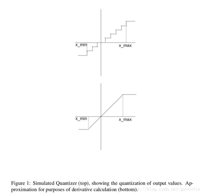
Since the derivative of a simulated uniform quantizer function is zero almost everywhere, approximations are required to model a quantizer in the backward pass. An approximation that has worked well in practice (see [5]) is to model the quantizer as specified in equation 14 for purposes of defining its derivative (See figure 1).
由于模拟的统一量化方程的导数几乎在各个位置均为0,我们需要在反向传播中构建一个近似量化。在实际工程中一种效果比较好的近似方法(参见[5])是将量化指定为公式14的形式,这样可以方便定义导数(参见图1).
The backward pass is modeled as a ”straight through estimator” (see [5]). Specifically,
反向传播可以建模为“直通估计器”,参见[5]。既
其中XXX是关于模拟的量化输出的loss的反向传播误差。
2.5 Determining Quantizer parameters
The quantizer parameters can be determined using several criteria. For example, TensorRT [11] minimizes the KL divergence between the original and quantized distributions to determine the step size. In this work, we adopt simpler methods. For weights,we use the actual minimum and maximum values to determine the quantizer parameters. For activations, we use the moving average of the minimum and maximum values across batches to determine the quantizer parameters. For post training quantization approaches, one can improve the accuracy of quantized models by careful selection of quantizer parameters.
量化参数可以利用一些标准来决定。例如,TensorRT[11]通过最小化原始数据分布和量化后数据分布之间的KL散度来决定步长尺度。在本文中,我们采用一些更简单的方法。对于权重,我们使用实际的最大和最小值来决定量化参数。对于激活输出,我们使用跨批(batches)的最大和最小值的滑动平均值来决定量化参数。对于先训练后量化的方法,我们可以通过仔细地选择量化参数来提高量化模型的精度。
2.6 Granularity of quantization
We can specify a single quantizer (defined by the scale and zero-point) for an entire tensor, referred to as per-layer quantization. Improved accuracy can be obtained by adapting the quantizer parameters to each kernel within the tensor [17]. For example, the weight tensor is 4 dimensional and is a collection of 3 dimensional convolutional kernels, each responsible for producing one output feature map. per-channel quantization has a different scale and offset for each convolutional kernel. We do not consider per-channel quantization for activations as this would complicate the inner product computations at the core of conv and matmul operations. Both per-layer and per-channel quantization allow for efficient dot product and convolution implementation as the quantizer parameters are fixed per kernel in both cases.
对于一个完整的张量,我们可以指定一个简单的量化器(由尺度∆和零点z定义)对其量化,定义为“逐层量化”。如果想让精度进一步提升,可以采用对张量的每个卷积核都使用对应的量化器[17]。例如,权重张量是4维的,是3维卷积核的一个集合,集合中每个成员都负责产生一个特征输出。“逐通道量化”对于每个卷积核都有不同的尺度和零点。对于激活输出我们不考虑逐通道量化,因为这会使卷积操作和矩阵乘操作中的内积计算变得复杂。“逐层量化”和“逐通道量化”都支持高效的点乘操作和卷积实现,因为这两种量化方式中量化参数在每个卷积核中都是固定的常量。
3 Quantized Inference: Performance and Accuracy
Quantizing a model can provide multiple benefits as discussed in section 1. We discuss multiple approaches for model quantization and show the performance impact for each of these approaches.
在第1小节中我们知道,量化一个模型可以有很多好处。现在我就讨论一下模型量化的各种方法,并展示各种方法之间的性能影响。
3.1 Post Training Quantization (训练后量化)
In many cases, it is desirable to reduce the model size by compressing weights and/or quantize both weights and activations for faster inference, without requiring to re-train the model. Post Training quantization techniques are simpler to use and allow for quantization with limited data. In this section, we study different quantization schemes for weight only quantization and for quantization of both weights and activations. We show that per-channel quantization with asymmetric ranges produces accuracies close to floating point across a wide range of networks.
在许多情况下,我们希望在不重新训练模型的前提下,只是通过压缩权重或量化权重和激活输出来缩减模型大小,从而加快预测速度。“训练后量化”就是这种使用简单,而且在有限的数据条件下就可以完成量化的技术。在本节中,我们开始研究不同的量化方案,包括“只对权重量化”和“对权重和激活输出都量化”。然后展示“非对称取值范围的逐通道量化”对于很多网络而言,都可以产生和浮点型很接近的精度。
3.1.1 Weight only quantization (只对权重量化)
A simple approach is to only reduce the precision of the weights of the network to 8-bits from float. Since only the weights are quantized, this can be done without requiring any validation data (See figure 2). A simple command line tool can convert the weights from float to 8-bit precision. This setup is useful if one only wants to reduce the model size for transmission and storage and does not mind the cost of performing inference in floating point.
一个简单的方法是只将权重的精度从浮点型减低为8bit整型。由于只有权重进行量化,所以无需验证数据集就可以实现。一个简单的命令行工具就可以将权重从浮点型转换为8bit整型。如果只是想为了方便传输和存储而减小模型大小,而不考虑在预测时浮点型计算的性能开销的话,这种量化方法是很有用的。
3.1.2 Quantizing weights and activations (量化权重和激活输出)
One can quantize a floating point model to 8-bit precision by calculating the quantizer parameters for all the quantities to be quantized. Since activations need to be quantized, one needs calibration data and needs to calculate the dynamic ranges of activations.(See figure 2) Typically, about 100 mini-batches are sufficient for the estimates of the ranges of the activation to converge.
我们可以通过计算所有将要被量化的数据的量化参数,来将一个浮点型模型量化为一个8bit精度的整型模型。由于激活输出需要量化,这时我们就得需要标定数据了,并且需要计算激活输出的动态范围。(参见图2)。一般使用100个小批量数据就足够估算出激活输出的动态范围了。
3.1.3 Experiments
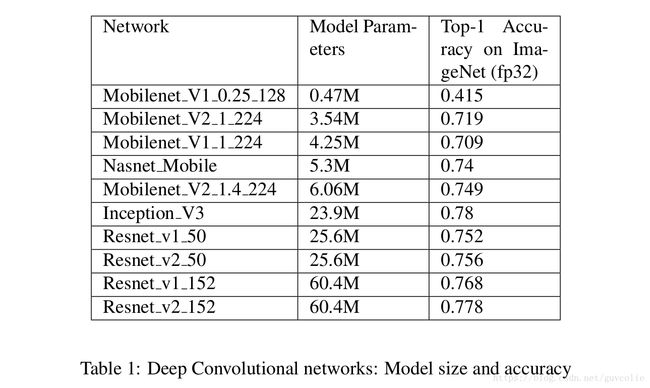
For evaluating the tradeoffs with different quantization schemes, we study the following popular networks and evaluate the top-1 classification accuracy. Table 1 shows the wide variation in model size and accuracy across these networks. We note that Mobilenet-v1 [2] and Mobilenet-v2[1] architectures use separable depthwise and pointwise convolutions with Mobilenet-v2 also using skip connections. Inception-v3 [18] and NasNet [19] use network in network building blocks with NasNet determining the
architecture via reinforcement learning techniques. Resnets [20] pioneered the idea of skip connections and consist of multiple blocks each making residual corrections to the main path with no transformations. Resnet-v2 [21] is an enhancement to the resnet architecture using pre-activation layers for improved accuracy. Note that all results are obtained using simulated quantization of weights and activations.
为了在不同的量化方案之间进行评估权衡,我们对以下常用的网络进行了研究,并评估了top-1分类精度指标。表1显示了这些模型之间,在模型大小和精度上相差很大。我们注意到Mobilenet-v1 [2] 和 Mobilenet-v2[1] 架构使用了separable depthwise and pointwise convolutions(可分离深度向及点向卷积),而且Mobilenet-v2 也使用了跳连操作。Inception-v3 [18] 和 NasNet [19] 使用了NasNet的network in network building blocks(网中网构建模块),其中NasNet是一种通过强化学习训练得到的一种全局搜索架构。Resnets [20] 首先提出了跳连思想,并包含了许多块,每个块都把残差修正直连到主路径中。Resnet-v2 [21] 是resnet结构的增强版,它为了精度进一步提升,使用了预输出层。注意,一下所有结果都是使用权重和激活输出的模拟量化而得到的。
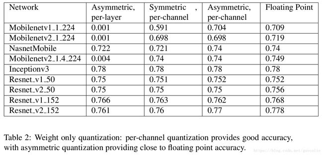
Weight only quantization: We first quantize only the weights post training and leave the activations un-quantized. From figure 2, we note that per-channel quantization is required to ensure that the accuracy drop due to quantization is small, with asymmetric, per-layer quantization providing the best accuracy.
只量化权重:我们首先只量化权重,激活输出暂时不进行量化。从图2可知,逐通道量化需要确保因量化而造成的精度下降要比较小,而且非对称、逐通道(原文写成per-layer,我认为它是写错了!)量化方式会产生最高的精度。
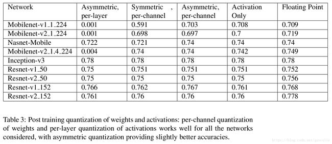
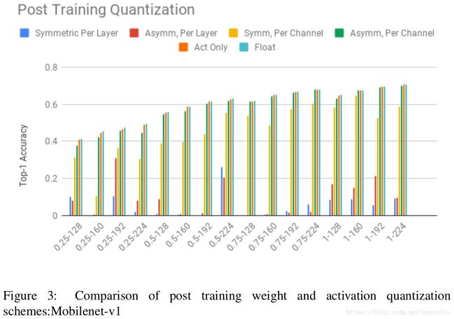
Weight and Activation Quantization: Next, we quantize weights and activations to 8-bits, with per-layer quantization for activations. For weights we consider both symmetric and asymmetric quantizers at granularities of both a layer and a channel. We first show results for Mobilenetv1 networks and then tabulate results across a broader range of networks.
量化权重和激活输出:接下来,我们将权重和激活输出量化为8bit,且对激活输出采用逐层量化的方式。对于权重,我们在逐层和逐通道两个粒度下考虑对称和非对称量化方案。我们首先展示Mobilenetv1的结果,然后在表格中对其他各个网络进行展示。
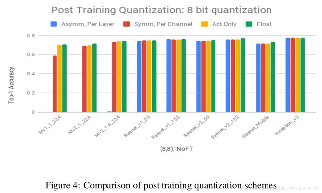
We also compare the post training quantization accuracies of popular convolutional networks: Inception-V3, Mobilenet-V2, Resnet-v1-50, Resnet-v1-152, Resnet-v2-50, Resnet-v2-152 and Nasnet-mobile on ImageNet in figure 4.
我们也比较了各个常用模型采用先训练后量化的量化精度,其中包括在ImageNet训练评测的Inception-V3, Mobilenet-V2, Resnet-v1-50, Resnet-v1-152, Resnet-v2-50, Resnet-v2-152 和 Nasnet-mobile的精度。
We make the following observations:
我们发现了如下规律:
1. Per-channel quantization can provide good accuracy and can be a good baseline for post training quantization of weights and activations, with asymmetric quantization providing close to floating point accuracy for all networks.
1. 逐通道量化方法可以提供很好的精度,可以作为权重和激活输出的先训练后量化的很好的基线,而且非对称量化方式对于所有模型都能提高和浮点型很相近的精度。
2. Activations can be quantized to 8-bits with almost no loss in accuracy. The dynamic ranges of the activations are low due to a combination of:
2. 激活输出做8bit量化后,精度几乎没有损失。由于以下原因,激活输出的动态范围一般很小:
- (a) Batch normalization with no scaling: Used in Inception-V3, which ensures that the activations of all feature maps have zero mean and unit variance.
- (a) 无缩放的批归一化:它可以确保所有特征的激活输出服从均值为0,方差为1的分布。
- (b) ReLU6: Used in Mobilenet-V1, which restricts the activations to be in a fixed range (0,6) for all feature maps, thereby removing large dynamic range variations.
- (b) ReLU6: 它可以将所有的特征输出都固定到(0, 6)范围内,从而消除大动态范围的可能。
3. Networks with more parameters like Resnets and Inception-v3 are more robust to quantization compared to Mobilenets which have fewer parameters.
3. 像Resnets 和 Inception-v3 这种有更多参数的模型与Mobilenets 这种参数较少的模型相比,对于量化的鲁棒性会更高。
4. There is a large drop when weights are quantized at the granularity of a layer, particularly for Mobilenet architectures.
4. 当采用逐层量化的方式对权重进行量化时,会有非常大的精度损失,尤其对于Mobilenet架构。
5. Almost all the accuracy loss due to quantization is due to weight quantization.
5. 几乎所有的量化精度损失都是源于权重量化而导致的。
Weight quantization at the granularity of a layer causes large accuracy drops primarily due to batch normalization, which causes extreme variation in dynamic range across convolution kernels in a single layer. Appendix A has more details on the impact of batch normalization. Per-channel quantization side-steps this problem by quantizing at the granularity of a kernel, which makes the accuracy of per-channel quantization independent of the batchnorm scaling. However, the activations are still quantized with per-layer symmetric quantization.
采用逐层量化的方式对权重进行量化时,会产生很大的精度损失,这是因为bn操作在特征层的各个通道间的动态范围差异非常大。Appendix A对bn产生的影响做了更详尽的讨论。逐层量化可以通过通道粒度来避免这个问题,它可以逐通道地量化而不依赖与bn的缩放。但是,激活输出仍然需要采用逐层对称量化方式来量化。
Note that other approaches like weight regularization can also improve the accuracy of quantization post training, please see [22].
其他的方法,比如像权重正则化,也可以对训练后量化提高量化精度,详见[22]。
3.2 Quantization Aware Training (训练时量化)
Quantization aware training models quantization during training and can provide higher accuracies than post quantization training schemes. In this section, we describe how quantization is modeled during training and describe how this can be easily done using automatic quantization tools in TensorFlow. We also evaluate the accuracies obtained for different quantization schemes with quantization aware training and show that even per-layer quantization schemes show high accuracies post training at 8-bits of precision. We also show that at 4 bit precision, quantization aware training provides significant improvements over post training quantization schemes.
训练时量化方法相比于训练后量化,能够得到更高的精度。在本节中,我们将阐述如何在训练过程中进行量化,以及如何利用Tensorflow的自动量化工具将量化很容易地完成。我们也会对训练时量化的不同量化方案进行评估,并展示甚至是采用逐层量化方案也能得到很高的精度。我们也展示,即使采用4bit训练时量化方案都比训练后量化的精度高。
We model the effect of quantization using simulated quantization operations on both weights and activations. For the backward pass, we use the straight through estimator (see section 2.4) to model quantization. Note that we use simulated quantized weights and activations for both forward and backward pass calculations. However, we maintain weights in floating point and update them with the gradient updates. This ensures that minor gradient updates gradually update the weights instead of underflowing. The updated weights are quantized and used for subsequent forward and backward pass computation. For SGD, the updates are given by:
我们对于权重和激活输出采用模拟量化操作来衡量量化效果。对于反向传播,我们使用“直通估计器”(见2.4节)去建模量化。注意,在前向和反向传播计算中,我们使用的都是模拟量化的权重和激活输出。但同时,我们也保留浮点型权重,并且在梯度更新的过程中更新它们。这样可以确保使用较小的梯度更新逐步更新权重,而不会造成梯度满溢。更新的权重被量化,然后用于后续的前向和反向传播计算。对于SGD(随机梯度下降),更新方式如下:
Quantization aware training is achieved by automatically inserting simulated quantization operations in the graph at both training and inference times using the quantization library at [23] for Tensorflow [24]. We follow the approach outlined in [4] closely, with additional enhancements on handling batch normalization and in modeling quantization in the backward pass. A simple one-line change to the training or evaluation code automatically inserts simulated quantization operations into the training or eval graph.
训练时量化方案可以利用Tensorflow的量化库,在训练和预测时在模型图中自动插入模拟量化操作来实现。我们主要采用[4]所阐述的方法,包括处理bn的增强和反向传播时的构建量化。在训练或预测的代码中只需要一行简单的修改就可以将模拟量化操作自动插入到训练或预测图中。
For training, the code snippet is:
对于训练,代码片段如下:
# Build forward pass of model.
...
loss = tf.losses.get_total_loss()

#Call the training rewrite which rewrites the graph in-place
#with FakeQuantization nodes and folds batchnorm for training.
#One can either fine tune an existing floating point model
#or train from scratch. quant_delay controls the onset
#of quantized training.

tf.contrib.quantize.create_training_graph(quant_delay=2000000)

# Call backward pass optimizer as usual.
optimizer = tf.train.GradientDescentOptimizer(learning_rate)
optimizer.minimize(loss)
For evaluation, the code snippet is given below:
对于测试,代码片段如下:
# Build eval model
...
logits, end_points = network_model(inputs,...)
# Call the eval rewrite which rewrites the graph in-place
# with FakeQuantization nodes and fold batchnorm for eval.
tf.contrib.quantize.create_eval_graph()
The high level conversion process is shown in figure 2.
高层转换过程如图2所示。
The steps involved in training a quantized model are:
在训练中,量化一个模型的步骤为:
- (Recommended): Fine tune from a floating point saved model: Start with a floating point pre-trained model or alternately train from scratch
- (建议)在保存好的浮点型模型的基础上精调:在预训练好的模型基础上继续训练或者重新训练
- Modify Estimator to add quantization operations: Add fake quantization operations to the model using the quantization rewriter at tf.contrib.quantize
- 修改估计器,添加量化运算:利用tf.contrib.quantize中的量化rewriter向模型中添加假的量化运算
- Train model: At the end of this process, we have a savedmodel with quantization information (scale, zero-point) for all the quantities of interest. (weights and activations)
- 训练模型:这个过程结束后,我们就拥有了一个对于权重和激活输出都带有各自量化信息(尺度、零点)的保存好的模型。
- Convert model: The savedmodel with range information is transformed into a flatbuffer file using the tensorflow converter (TOCO) at: tf.contrib.lite.toco convert. This step creates a flatbuffer file that converts the weights into integers and also contains information for quantized arithmetic with activations
- 转换模型:利用Tensorflow的在 tf.contrib.lite.toco convert定义的转换器,将带有量化参数的模型被转化成一个flatbuffer文件。这步会产生一个flatbuffer文件,这个文件会将权重转换成int整型,同时包含了激活输出用于量化计算的信息
- Execute model: The converted model with integer weights can now be executed using the TFLite interpreter which can optionally execute the model in custom accelerators using the NN-API. One can also run the model on the CPU.
- 执行模型:转换后的带有整型权重的模型可以利用TFLite interpreter来执行,也可以在CPU上运行模型
A simple example showing the graph transformation for a convolutional layer is shown in figure 5.
一个简单的卷积层的转图例子参见图5.
3.2.1 Operation Transformations for Quantization
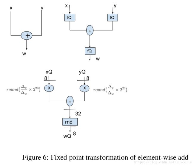
It is important to ensure that all quantization related artifacts are faithfully modeled at training time. This can make trivial operations like addition, figure 6 and concatenation , figure 7 non-trivial due to the need to rescale the fixed point values so that addition/concatenation can occur correctly.
确保在训练时所有与量化相关的人为操作都如实地进行建模是非常重要的。这可以使简单的操作,比如add(图5)和concat(图6)操作,变得有意义,因为需要重新调整定点值以使这些操作能够正确地工作。
In addition, it is important to ensure that fusion of operations at inference time is modeled correctly during training. For example, consider an add followed by a ReLU operation. In this case, one can fuse the addition and the ReLU operation at inference time in most platforms. To match this, fake quantization operations should not be placed between the addition and the ReLU operations.
除此之外,在训练期间确保在预测时操作符的融合能够正确地建模是很重要的。例如,考虑一个add操作,然后紧跟一个ReLU操作。在这种情况下,大多数硬件平台都支持在预测阶段将add和ReLU进行融合。为了匹配这种情况,假的量化操作运算不应该置于add和ReLU之间。
3.2.2 Batch Normalization
In this section, we describe several strategies for quantizing batch normalization layers. In section 4 and show that batch normalization with correction and freezing provides the best accuracy.
在本小节中,我们描述一些量化BN层的采取的策略。第4小节会展示带有纠正和冻结的bn会得到最高的精度。
Batch normalization [25], is a popular technique that normalizes the activation statistics at the output of every layer, reducing dependencies across layers while significantly improving model accuracy.
Batch normalization是一个很受欢迎的技术,它可以将每层输出的各个通道统计量进行归一化,在很好地提升模型精度的同时,也可以降低层间依赖。
Batch normalization is defined by the following equations:
在训练阶段,Batch normalization定义如下:
在预测阶段,Batch normalization定义如下:
Where μ B and σ B are the batch mean and standard deviations. μ and σ are the long term mean and standard deviations and are computed as moving averages of batch statistic during training.
其中 μ B 和 σ B分别为batch的均值和标准差。μ 和 σ 是整个训练集的均值和标准差,在训练阶段,这两个值可以通过batch的滑动平均方式计算得到(感兴趣的朋友可以自行了解momentum知识)。
For inference, we fold the batch normalization into the weights as defined by equations 20 and 21. Therefore, at inference there is no explicit batch normalization. The weights and biases are modified to account for batch normalization instead:
对于预测,我们将bn按照公式21和22所定义的那样折叠进权重中。因此,在预测时没有显式的bn操作。bn按如下方式拆分整合为权值和偏置:
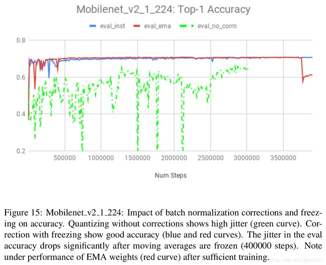
For quantized inference, we first consider folding batch norms and training them as shown in figure 8. We note that batch normalization uses batch statistics during training, but uses long term statistics during inference. Since the batch statistics vary every batch, this introduces undesired jitter in the quantized weights and degrades the accuracy of quantized models. (green curve in 14 and 15) A simple solution would be to switch to using long term moving averages during training, however, this eliminates batch normalization (i.e the mean and variance used do not correspond to the batch statistics) and causes instability in training. The graph rewriter implements a solution that eliminates the mismatch between training and inference with batch normalization(see figure 9):
对于量化预测,我们首先考虑折叠bn并像图8所示那样训练。我们注意到在训练阶段bn会使用batch批统计信息(既batch均值和方差),而在预测阶段使用的是整个训练集的均值和标准差。由于批统计量在每个batch批之间变化很大,这会在量化的权重中引入不希望的跳变,也会是量化模型的精度降低。(图14、15中绿线所示)。一个简单的解决方法是,在训练时也使用整个训练集的均值和标准差,但是这样会使“!批!”归一化失去意义(既均值和标准差和批统计量完全没有了关系),并且会导致训练不稳定。图重构也是一种解决方法,它可以消除训练和预测时bn的差异(如图9所示):
1. We always scale the weights with a correction factor to the long term statistics prior to quantization. This ensures that there is no jitter in the quantized weights due to batch to batch variation.
1. 我们需要先于量化之前在完整训练集统计量上乘以一个带修正因子的权重。这会确保即使存在批统计量波动,量化权重也不会出现跳变。
2. During the initial phase of training, we undo the scaling of the weights so that outputs are identical to regular batch normalization. We also modify the bias terms correspondingly.
2. 在训练的初始阶段,不做权重的缩放(1步骤提到的),这样输出就是常规bn的输出。偏置bias同理。
3. After sufficient training, switch from using batch statistics to long term moving averages for batch normalization, using the optional parameter freeze_bn_delay in create_experimental_training_graph() (about 300000 steps in figure 15 and 200000 in figure 14). Note that the long term averages are frozen to avoid instability in training. This corresponds to the normalization parameters used at inference and provides stable performance.
3. 在经过充分训练后(图15大约训练300000步,图14大约训练200000步),利用create_experimental_training_graph()中的可选参数freeze_bn_delay,将批统计量(均值、标准差)替换为此时计算得到的训练集统计量(均值、标准差)。注意这时需要将训练集统计量(均值、标准差)冻结,从而避免训练不稳定。这相当于预测时使用的归一化参数,可以保证相对稳定的性能。
3.2.3 Experiments
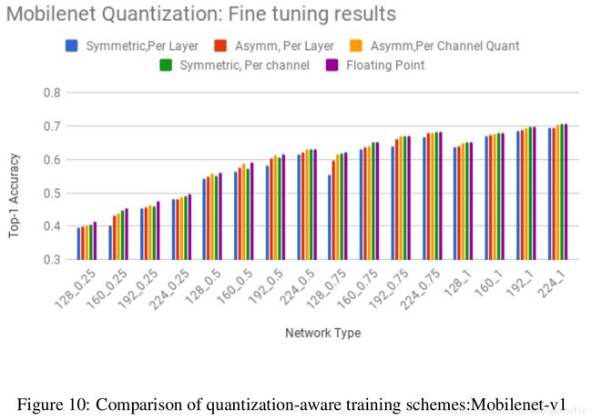
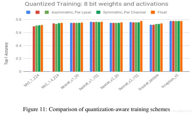
Quantization aware training closes the gap to floating point accuracy, even for per-layer quantization of weights. We repeat the same experiments for quantized weights and activations with training, starting from a floating point check-point and with batch normalization freezing and obtain the results shown in figures 11 and 10 and Table 4.
训练时量化精度和浮点型模型精度相差无几,甚至对于权重的逐层量化方式也是如此。我们在训练中,重复做了之前的对权重和激活输出的量化实验,我们从浮点型checkpoint继续训练,并将bn冻结,得到的结果如图11、12和表4所示。
All the experiments have the following settings:
所有实验都采用以下设置:
- Fine tune from a floating point checkpoint, we used the models in [26].
- 从浮点型checkpoint继续训练,我们使用[26](slim官方预训练模型)中提高的模型。
- Use Stochastic Gradient Descent for fine tuning, with a step size of 1e-5.
- 使用随机梯度下降法训练,学习率1e-5.
We note that:
我们发现:
1. Training closes the gap between symmetric and asymmetric quantization.
1. 采用对称量化和非对称量化的训练结果相差很小。
2. Training allows for simpler quantization schemes to provide close to floating point accuracy. Even per-layer quantization shows close to floating point accuracy (see column 4 in Table 4)
2. 即使采用很简单的量化方案,也能达到几乎和浮点型精度一样的精度。甚至逐层量化也是如此。(参见表4第4列)
3.2.4 Lower Precision Networks
We note that at 8-bits of precision, post training quantization schemes provide close to floating point accuracy. In order to better understand the benefits of quantization aware training, we perform experiments to assess performance at 4 bit quantization for weights and activations.
在8bit精度上,训练后处理方案的精度和浮点型精度模型相差很小。为了能够更好地理解训练时量化所带来的好处,我们对权重和激活输出做了4bit量化实验,并验证了性能。
We perform the following experiments:
我们做了如下实验:
- Experiment 1: Per-channel quantization is significantly better than per-layer quantization at 4 bits. We show that per-channel quantization provides big gains over per-layer quantization for all networks. At 8-bits, the gains were not significant as there were sufficient levels to represent the weights with high fidelity. At four bits, the benefits of per-channel quantization are apparent, even for post training quantization (columns 2 and 3 of Table 5).
- 实验1:在4bit精度上,逐通道量化明显要比逐层量化精度要高。实验显示对于所有的模型,逐通道量化都优于逐层量化。在8bit精度上,差距就没那么明显了,因为模型有足够的bit位容量,可以以高保真度去表征权重。在4bit精度,逐通道量化的好处还是很明显的,甚至对于训练后量化也是如此。(参见表5的第2、3列)
- Experiment 2: Fine tuning can provide substantial accuracy improvements at lower bitwidths. It is interesting to see that for most networks, one can obtain accuracies within 5% of 8-bit quantization with fine tuning 4 bit weights (column 4 of Table 5). The improvements due to fine tuning are also more apparent at 4 bits. Note that activations are quantized to 8-bits in these experiments.
- 实验2:在低的bit位宽情况下,在已有模型基础上继续训练会大幅提升模型精度。我们发现一个有趣的现象,对于大多数网络来讲,采用4bit位宽精调得到的精度结果也只是比8bit量化的精度小5%以内(参见表5的第4列)。对于4bit位宽,在已有模型基础上继续训练(精调)所带来的精度提升更加冥想。注意,在这些实验中,激活输出仍采用8bit量化方式。
- Experiment 3: Lower precision activations: We investigate the accuracies obtained with 4-bit activations for all layers with and without fine tuning. Note that activations are quantized on a per-layer basis. The weights are quantized at 8-bits of precision with per-channel granularity. We note that fine tuning improves accuracy in this case also. The losses due to activation quantization are more severe than that of weight quantization (see Table 6). Note that the quantization granularity is different for activations and weights, so this is not a fair comparison of the impact of quantization. We hypothesize that quantizing activations introduces random errors as the activation patterns vary from image to image, while weight quantization is deterministic. This allows for the network to learn weight values to better compensate for the deterministic distortion introduced by weight quantization.
- 实验3:更低精度的激活输出量化:我们分别在精调和不精调的条件下,对所有层的激活输出采用4bit量化的精度进行了研究。注意,这里激活输出采用逐层量化,而权重采用8bit逐通道量化。我们发现在这些实验中精调也会提升模型精度。激活输出的量化损失要比权重量化的精度损失多得多(参见表6)。注意权重和激活输出的量化粒度是不同的,所以对于量化影响来讲其实这不是一个公平的比较。所以我们只能猜测表6结果的原因是,量化激活输出会引入随机误差,因为不同图片之间的激活输出是有较大差异的,而权重量化是确定的,这就使网络能够更好地学习权重,从而补偿权重量化所带来的计算偏差。
4 Training best practices (训练最佳实践)
We experiment with several configurations for training quantized models: Our first experiment compares stochastic quantization with deterministic quantization. Subsequently, we study if training a quantized model from scratch provides higher accuracies than fine tuning from a floating point model. We also evaluate different methods for quantizing batch normalization layers and show that batch normalization with corrections provides the best accuracy. We also compare schemes that average weights during training with no averaging.
我们做了一些不同配置的训练量化模型的实验:首先,我们比较了随机量化(2.3节)和确定性量化(2.3节之外的量化方式)。然后,我们研究了从头开始训练一个量化模型所得到的模型精度是否会比从浮点型checkpoint基础上训练得到的模型精度要高。我们也对量化bn的不同方法进行的评测,结果显示带有修正的bn会产生最好的精度。我们也比较了在训练中对权重进行平均和不进行平均这两种方案。
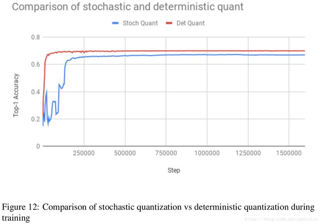
1. Stochastic Quantization does not improve accuracy: Stochastic quantization determines floating point weights that provide robust performance under stochastic quantization, which causes the quantized weights to vary from mini-batch to mini-batch. At inference, quantization is deterministic, causing a mismatch with training. We observe that due to this mis-match, stochastic quantization underperforms determinstic quantization (figure 12), which can be compensated better during training.
1. 随机量化不会提升精度:随机量化方案会确定浮点型权重,这种浮点型权重在随机量化中提供鲁邦的性能,但这样会导致量化的权重在小批量之间波动变化。在预测时,量化值是确定的,这就会导致和训练时的不一致。我们发现正是因为这种不一致,会导致随机量化方案和确定量化方案相比表现不佳(图12),因为确定量化方案在训练过程中能够更好地补偿这种不一致。
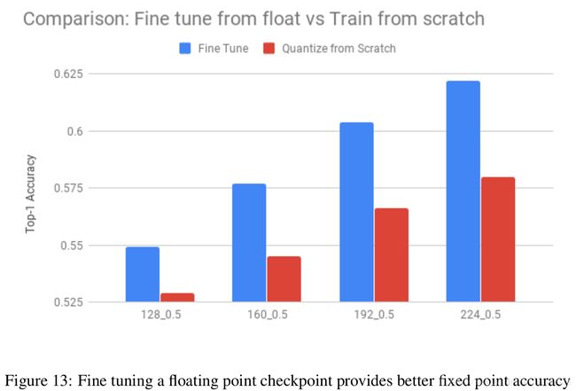
2. Quantizing a model from a floating point checkpoint provides better accuracy: The question arises as to whether it is better to train a quantized model from scratch or from a floating point model. In agreement with other work [27], we notice better accuracy when we fine tune a floating point model as shown in figure 13. This is consistent with the general observation that it is better to train a model with more degrees of freedom and then use that as a teacher to produce a smaller model ([28]).
2. 在浮点型checkpoint基础上量化模型会得到更好的精度:这个问题实际上就是从头开始训练一个量化模型所得到的模型精度是否会比从浮点型checkpoint基础上训练得到的模型精度要高。和其他的研究成果[27]一致,我们发现从浮点型checkpoint基础上继续训练模型会得到更好的精度,如图13。这也和一般的发现规律——最好先以尽可能多的自由度去训练一个模型,然后用这个模型作为引导老师去训练更小的模型——相一致。
3. Matching Batch normalization with inference reduces jitter and improves accuracy. We show results for two networks. In the first experiment (see figure 14), we compare training with naive batch norm folding, batch renormalization and batch normalization with correction and freezing for Mobilenet-v1_1_224. We note stable eval accuracy and higher accuracy with our proposed approach. In the second experiment, we compare naive batch norm folding and batch normalization with correction and freezing for Mobilenet-v2_1_224. We note that corrections stabilize training and freezing batch norms provides additional accuracy gain, seen after step 400000 in figure 15.
3. 将bn结构按预测进行匹配会降低数据抖动,提高模型精度。我们展示两个网络的结果。在第一个实验中(图14),我们利用Mobilenet-V1_1_224比较了原始实现的bn和采用纠正和冻结方式的bn。我们发现采用我们提出的方法能得到更稳定、更高的精度。在第二个实验中,我们利用Mobilenet-V2_1_224比较了原始实现的bn和采用纠正和冻结方式的bn。我们发现纠正操作可以稳定训练,冻结可以是精度进一步提升,参见图15中400000步后。
4. Use Exponential moving averaging for quantization with caution. Moving averages of weights [29] are commonly used in floating point training to provide improved accuracy [30]. Since we use quantized weights and activations during the back-propagation, the floating point weights converge to the quantization decision boundaries. Even minor variations in the floating point weights, between the instantaneous and moving averages can cause the quantized weights to be significantly different, hurting performance, see drop in accuracy for the EMA curve in figure 15.
4. 慎用指数滑动平均。在浮点型模型训练中,为了提高精度[30],通常会对权重进行滑动平均操作[29]。由于我们在反向传播时使用的是量化后的权重和激活输出,浮点型权重可能会收敛于量化决策边界的位置上。甚至,瞬时的和滑动平均的浮点型权重之间的微小差异,也会导致量化的权重产生非常明显的不同,这会影响性能,参见图15中EMA(Exponential moving averaging)指数滑动平均对应曲线的精度下降。
5 Model Architecture Recommendations (模型架构建议)
In this section, we explore choices of activation functions and tradeoffs between precision and width of a network.
在本节中,我们探讨激活函数的选择,以及模型精度和模型宽度(其实就是模型尺寸)之间的取舍问题。
- Do not constrain activation ranges: One can get slightly better accuracy by replacing ReLU6 non-linearity with a ReLU and let the training determine the activation ranges (see figure 16)
- 不要约束激活范围:将ReLU6替换为ReLU,会有微小的精度提升,所以就让模型在训练中自己确定激活范围吧(参见图16)
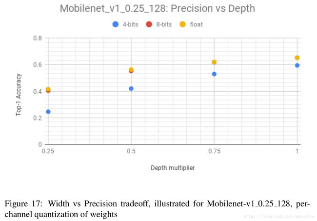
- Explore tradeoff of width vs quantization: An over-parameterized model is more amenable to quantization. Even for leaner architectures like mobilenet, one can tradeoff the depth multiplier with the precisions of the weights. We compare the accuracies obtained with 4 bit per-channel quantization of weights with 8-bit quantization across different depth multipliers in figure 17. Note that this comparison allows us to evaluate a depth vs quantization tradeoff (see [31]). It is interesting to see that one can obtain a further 25% reduction in the model size for almost the same accuracy by moving to 4 bit precision for the weights.
- 探索模型宽度和量化之间的取舍:冗余度较高的模型更适合量化。即使对于想mobilenet这种更加精简的模型架构,也可以在精度和模型尺寸之间进行取舍。我们拿4bit权重逐通道量化模型 和 8bit不同深度乘子的量化模型(也就是8bit不同容量的量化模型),针对精度进行了比较,如图17。这种比较允许我们评估一种容量和量化之间的权衡关系(参见[31])。我们发现一个有趣的现象,将权重进行4bit量化后的模型精度 和 直接将模型容量缩减25%的模型精度相差无几。
6 Run-time measurements (运行时间测量)
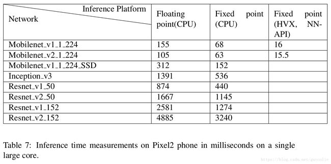
We measure the run-times (Table 7) on a single large core of the Google Pixel 2 device for both floating point and quantized models. We also measure run-times using the Android NN-API on Qualcomm’s DSPs. We see a speedup of 2x to 3x for quantized inference compared to float, with almost 10x speedup with Qualcomm DSPs.
我们在Google Pixel 2手机上利用单个大核,分别测量了浮点型模型和量化模型的运行时间,如表7所示。我们也在骁龙DSP上使用Android NN-API测量了运行时间。在Google Pixel 2上,量化模型的预测速度比浮点型模型的预测速度快2到3倍;在骁龙DSP上,会快大概10倍。
7 Neural network accelerator recommendations (神经网络加速器建议)
In order to fully realize the gains of quantized networks, we recommend that neural network accelerators consider the following enhancements:
为了让量化模型充分发挥其能力,建议神经网络加速器包含以下增强:
1. Aggressive operator fusion: Performing as many operations as possible in a single pass can lower the cost of memory accesses and provide significant improvements in run-time and power consumption.
1. 极致的运算符融合:在一次计算中,尽可能多地执行运算符,这样可以降低内存使用量、缩减运行时间以及减少耗电量。
2. Compressed memory access: One can optimize memory bandwidth by supporting on the fly de-compression of weights (and activations). A simple way to do that is to support lower precision storage of weights and possibly activations.
2. 压缩内存使用: 通过利用权重和激活输出的快速解压缩,我们可以优化内存带宽。实现这个操作的一个简单的方法就是去支持权重的低精度存储,甚至是激活输出。
3. Lower precision arithmetic: One can obtain further acceleration by supporting a range of precisions for arithmetic. Our recommendation is to support 4,8 and 16-bit weights and activations. While 4 and 8-bit precisions are sufficient for classification, higher precision support is likely needed for regression applications, like super-resolution and HDR image processing.
3. 低精度计算: 通过支持一系列精度的计算,可以进一步加速。我们的建议是支持4bit、8bit和16bit权重和激活输出。4bit和8bit精度对于分类任务来讲足够了,回归任务需要更高精度的支持,比如超分辨率和高动态范围图像处理。
4. Per-layer selection of bitwidths: We expect that many layers of a network can be processed at lower precision. Having this flexibility can further reduce model size and processing time.
4. 位宽逐层选择:我们期望网络的许多层可以在更低位宽精度下处理。这样做可以进一步减少模型尺寸和运行时间。
5. Per-channel quantization: Support for per-channel quantization of weights is critical to allow for:
(a) Easier deployment of models in hardware, requiring no hardware specific fine tuning.
(b) Lower precision computation.
5. 逐通道量化:支持逐通道量化对于以下几点的实现是至关重要的:
(a) 为了使模型在硬件上更容易部署,不需要特定硬件的精
(b) 更低精度计算
8 Conclusions and further work
Based on our experiments, we make the following conclusions:
基于我们的实验,做如下总结:
• Quantizing models
1. Use symmetric-per-channel quantization of weights with post training quantization as a starting point. Optionally fine tune if there is an accuracy drop.
1. 如果选择训练后量化策略,请使用权重的对称逐通道量化作为开始。如果精度有下降的话,可以考虑精调(在浮点型checkpoint基础上继续训练)
2. Quantization aware training can narrow the gap to floating point accuracy and in our experiments, reduce the gap to within 5% of 8-bit quantized weights, even when all layers are quantized to 4 bits of precision.
2. 训练时量化可以进一步减小和浮点型模型的精度差距,采用8bit量化时可以将精度差距缩减到5%以内,甚至当4bit量化所有层时也是如此。
• Performance
1. Quantized inference at 8-bits can provide 2x-3x speed-up on a CPU and close to 10x speedup compared to floating point inference on specialized processors optimized for low precision wide vector arithmetic, like the Qualcomm DSP with HVX.
1. 在CPU上,8bit量化预测可以提速2到3倍。在特定的专门为低精度向量计算优化过的处理器上,例如支持HVX的骁龙DSP,和浮点型模型预测速度相比可以提速近10倍。
2. One can obtain a model size reduction of 4x with no accuracy loss with uniform quantization. Higher compression can be obtained with non-uniform quantization techniques like K-means ([6]).
2. 我们利用均匀量化可以在精度不变的情况下将模型尺寸缩小4倍。更高的压缩可以通过非均匀量化技术实现,比如K-means[6]。
• Model architectures for quantization
1. There is a clear tradeoff between model size and compressibility. Larger models are more tolerant of quantization error.
1. 在模型尺寸和压缩比之间存在比较清晰的折中关系。容量越大的模型对量化误差的容忍度越高。
2. Within a single architecture, one can tradeoff feature-maps and quantization, with more feature maps allowing for lower bitwidth kernels.
2. 对于某一个模型结构,我们可以在特征数量和量化之间进行折中,要是用更多的特征数量就可以相应更低位宽的卷积核。
3. One can obtain improved accuracy by not constraining the ranges of the activations during training and then quantizing them, instead of restricting the range to a fixed value. In our experiments, it was better to use a ReLU than a ReLU6 for the activations.
3. 在训练中不约束激活函数的输出范围,然后直接对输出进行量化,这样会得到更高的精度。从我们的实验结果看出,对于激活输出最好使用ReLU,而不建议ReLU6。
Going forward, we plan to enhance our automated quantization tool to enable better quantization of networks by investigating the following areas:
1. Regularization techniques to better control the dynamic ranges of weights and activations can provide further improvements.
2. Distilled training to further improve the accuracy of quantized models [32].
3. Per-layer quantization of weights and activations to provide further compression and performance gains on hardware accelerators. Reinforcement learning has been applied successfully towards this problem in [33].
上面是Google对于量化工作后续的计划,我就不管了。
9 Acknowledgements
This work builds on the quantization scheme first introduced in [4]. Suharsh Sivakumar developed the [23] tool used for the quantization experiments, which extend the capabilities first described in [4]. Rocky Rhodes provided the performance measurement numbers for the models. We would also like to thank Cliff Young, Song Han, Rocky Rhodes and Skirmantas Kligys for their useful comments. Pete Warden provided useful input on the scope of the paper and suggested several experiments included in this document.
感谢... 感谢天~感谢地~感谢命运~让我们相遇~
References
引用请详见本文的pdf原文档
A Impact of Batch Normalization on Quantization
To understand the impact of batch normalization on the dynamic range of the folded weights (W), we consider the following metrics:
为了理解batch normalization对折叠权重W动态范围的影响,我们考虑如下指标:
1. SQNR: We calculate the Signal to quantization noise ratio defined as:
for different quantization schemes. We note that per-channel quantization provides significant improvement in SQNR over per-layer quantization, even if only symmetric quantization is used in the per-channel case.
1. SQNR: 对于不同的量化方案,我们定义“信号量化噪声比”为上式。我们发现逐通道量化在SQNR指标上比逐层量化效果好很多,甚至即使对称量化应用在逐通道量化情况下也是如此。
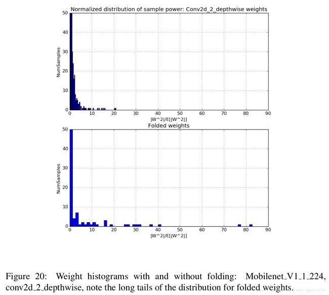
2. Weight Power Distribution: We also plot the distribution of the sample weights, normalized by the average power, i.e we plot
for the weights before and after folding. We note that after folding, there are much larger outliers which severely degrade performance.
2. 权重能量分布:我们也绘制了 利用平均能量归一化后的样本权重的分布,即我们为折叠前的权重和折叠后的权重绘制了分布图。我们发现在折叠后,存在很多严重降低性能的离散点。


