统计学习笔记(1) 监督学习概论(1)
原作品:The Elements of Statistical Learning Data Mining, Inference, and Prediction, Second Edition, by Trevor Hastie, Robert Tibshirani and Jerome Friedman
An Introduction to Statistical Learning. by Gareth JamesDaniela WittenTrevor Hastie andRobert Tibshirani
Brief Introduction to Statistical Learning
Suppose that we are statistical consultants hired by a client to provide advice on how to improve sales of a particular product. The Advertising data set consists of the sales of that product in 200 different markets, along with advertising budgets for the product in each of those markets for three different media: TV, radio, and newspaper. We want to increase the sales of the product by controling the advertising expenditure in each of the three media. So we determine the associations between medias and sales.
In this setting, the advertising budgets are input variables while sales input is an output variable. The input variables are typically denoted using the variable output variable symbol X, with a subscript to distinguish them. So X1 might be the TV budget, X2 the radio budget, and X3 the newspaper budget. The inputs go by different names, such as predictors, independent variables, features, predictor independent variable feature or sometimes just variables. The output variable—in this case, sales—is variable often called the response or dependent variable, and is typically denoted response dependent variable using the symbol Y .
Reducible and irreducible error
For quantitative response Y and different predictors X1, ... Xp. We assume that there is some
relationship between Y and X=(X1,X2,...,Xp), and make predictions based on input vector X and get result Y:
The second term is random error with mean zero and is independent of X.
Interpretations on f:
Sales is a response or target that we wish to predict. We generically refer to the response as Y . TV is a feature, or input, or predictor; we name it X1. Likewise name Radio as X2, and so on.
There is an ideal f(X). In particular, what is a good value for f(X) at any selected value of X, say X = 4? There can be many Y values at X = 4. A good value is f(4) = E(Y |X = 4) E(Y |X = 4) means expected value (average) of Y given X = 4. This ideal f(x) = E(Y |X = x) is called the regression function.
We can understand this as, we use the same input x to make several predictions: f1(x), f2(x),..., fm(x), the predictions are still different although the input keeps unchanged, due to distribution. The statistical average value of f1(x), f2(x),..., fm(x) will be our known correct result f(x) and also is the statistical value of Y. So we can make prediction:
![]()
(Different components in X have different importance). E(Y|X=x) means expected value (average) of Y given X=x. This ideal f(x)=E(Y|X=x) is called the regression function.
We can certainly make errors in prediction, the error is divided into 2 parts: one is reducible and the other is irreducible. The bias can be reduced, but the variance cannot.

This error is reducible because we can potentially improve the accuracy of fˆ by using the most appropriate statistical learning technique to estimate f. The quantity![]() may contain unmeasured variables that are useful in predicting Y: since we don’t measure them, f cannot use them for its prediction.
may contain unmeasured variables that are useful in predicting Y: since we don’t measure them, f cannot use them for its prediction.
Parametric and Non-parametric methods
We can apply parametricmodels
![]()
But Any parametric approach brings with it the possibility that the functional form used to estimate f is very different from the true f.
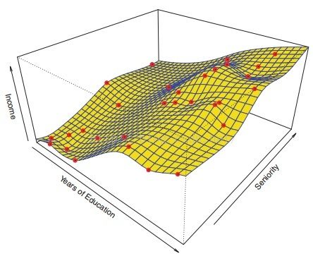
So we can use interpolation. Such as thin-plate spline. In order to fit a thin-plate spline, the data analyst must select a level of smoothness.
But overfitting might occur. To avoid overfitting, refer to Resampling Methods in "An Introduction to Statistical Learning" (Introduction to thin-plate splines: paper "Thin-Plate Spline Interpolation" on SpringerLink and code onhttp://elonen.iki.fi/code/tpsdemo/).
Trade-offs between Prediction Accuracy and Model Interpretability in curve fitting
Several considerations when choosing models:
1. Linear models are easy interpret while thin-plate splines are not.
2. Good fit Versus Overfitting.
3. We often prefer a simpler model involving fewer variables over a black-box predictor involving them all.
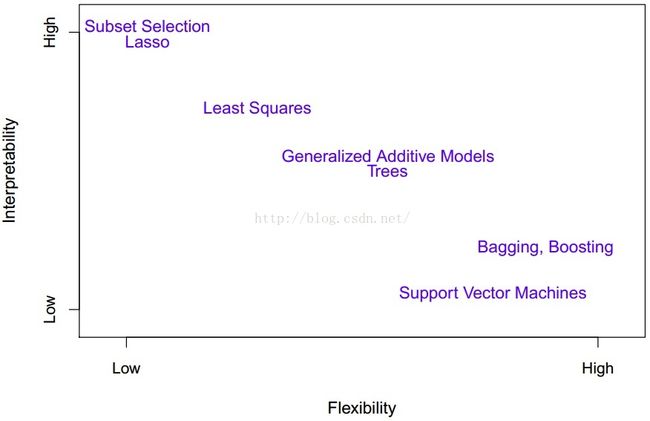
Following is a representation of the tradeoff between flexibility and interpretability, using different statistical learning methods. In general, as the flexibility of a method increases, its interpretability decreases.
Methods in assessing model accuracy:
MSE:
i is the index of observation. We use add in the test set. In practice, we use
the average squared prediction error for these test observations (x0, y0).
Choosing test data:
How can we go about trying to select a method that minimizes the test MSE? In some settings, we may have a test data set available—that is, we may have access to a set of observations that were not used to train the statistical learning method.
Evaluate model:
We choose 3 examples:
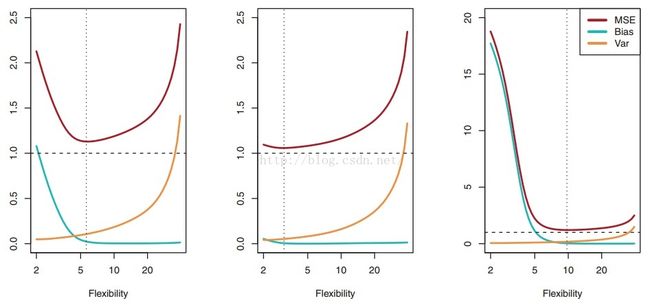
The first figure represents a comprehensive example, with high fluctuation and high noise level. The second figure has low fluctuation but high noise level, the third has high fluctuation and low noise level.
The horizontal dashed line indicates ![]() , which corresponds to the lowest achievable test MSE among all methods, as is shown in the following graphs, training errorcan be lower than the bound, but test errorcannot.
, which corresponds to the lowest achievable test MSE among all methods, as is shown in the following graphs, training errorcan be lower than the bound, but test errorcannot.
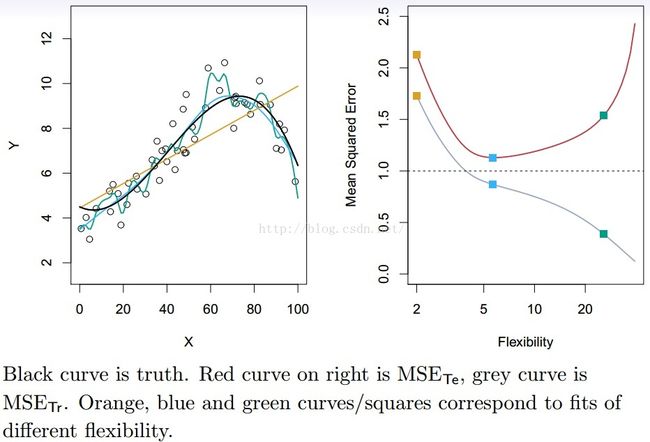
When we try to avoid overfitting by selecting the fresh test data, we find that the fluctuation influences the performance when fitting dimension (flexibility) is low, compare the second figure with the third figure, compare their low-flexibility parts, we can see if fluctuation increases, model with low flexibility cannot deal well, and in the third figure, as the flexibility increases from low values, the mean square error decreases, this is the advantage of high flexibility. From the second point of view, we compare the second figure with the third figure, the second figure suffers from strong noise while the third figure suffers from weak noise, when the flexibility (dimension of model) is very high, we can see from the second image that it fits to the noise well, but it's useless and it's overfitting, we can see when the noise is weak, too high flexibility is almost useless in the third figure. So a moderate in the middle will be enough. The red curve represents the error evaluated on the fresh test set, the gray curve represents the error evaluated on the training set.
Bias-Variance Trade-off
Suppose we have fit a model f^(x) to the training set. The true model is
with f(x)=E(Y|X=x), and
The left side of equal mark represents the expected test MSE. Refers to the average test MSE that we would obtain if we repeatedly estimated test MSE f using a large number of training sets and calculate theaverage value.
Variance: Variance refers to the amount by which fˆ would change if we estimated it using a different training data set. If a method has high variance, then small changes in the training set can result in large changes in f^.
Bias
Bias refers to the error that is introduced by approximating a real-life problem, which may be extremely complicated, by a much simpler model. For example, linear regression assumes that there is a linear relationship between Y and X1, X2, . . . , Xp. It is unlikely that any real-life problem truly has such a simple linear relationship, and so performing linear regression will undoubtedly result in some bias in the estimate of f.
As the flexibility (order of model) increases, the variance of estimation increases, the bias decreases. So choosing the flexibility based on average test error amounts to a bias-variance trade-off.
Corresponding to the above 3 graphs, blue-squared bias, orange-variance, red-test MSE, dashed line-![]() .
.
To help us evaluat test MSE with only training data, we can refer to cross validation in "Resampling Methods".
Classification
Suppose that we seek to estimate f on the basis of training observations {(x1, y1), . . . , (xn, yn)}, where now y1, . . . , yn arequalitative. Training error rate:
Bayes Classifier:
It is possible to show that the test error rate given is minimized, on average, by a very simple classifier that assigns each observation to the most likely class.
As to classification problems, consider a classifier C(X) that assigns a class label to observation X. Denote
The Bayes optimal classifier is (plot)
Typically we measure the estimation performance using
The Bayes classifier has smallest error.
SVMs build structured models for C(x), we also build structured models for representing the pk(x), e.g. Logistic regression, generalized additive models, K-nearest neighbors.


