医疗影像的图像处理基础
医疗影像的图像处理基础
介绍
在第一个任务中,我们将实现并应用一些基本的图像处理技术,以此来熟悉一些医学影像数据。
特别是我们将使用以下数据:
- mammography (breast, 2D)
- histopathology (colon, 2D)
- chest CT (lungs, 3D)
将实现下面的技术:
- 将原始的乳腺X片数据转为灰度图片
- 用直方图匹配对病历切片图像归一化
Libraries
首先导入我们这个任务所需要的库文件
import requests
import zipfile
from tqdm import tnrange, tqdm_notebook
import os
import SimpleITK as sitk
import matplotlib
import matplotlib.pyplot as plt
from matplotlib import cm
%matplotlib inline
import numpy as np
from PIL import Image
import dicom
from IPython import display
import time
from mpl_toolkits.mplot3d import Axes3D
import copy
matplotlib.rcParams['figure.figsize'] = (20, 17)
import scipy.signal
乳腺X光片灰度图变换
第一项任务包括从乳腺X光片机获取的原始数据,重建灰度乳腺X光图像。 必须采用几个步骤来重建灰度图像,从而使得放射科医生可以阅读这些图像,目的是检测肿瘤,肿块,囊肿,微钙化。
读取图片列表
# raw and gray-level data in ITK format
raw_img_filename = './assignment_1/raw_mammography.mhd'
out_img_filename = './assignment_1/processed_mammography.mhd'

# read ITK files using SimpleITK
raw_img = sitk.ReadImage(raw_img_filename)
out_img = sitk.ReadImage(out_img_filename)

# print image information
print('image size: {}'.format(raw_img.GetSize()))
print('image origin: {}'.format(raw_img.GetOrigin()))
print('image spacing: {}'.format(raw_img.GetSpacing()))
print('image width: {}'.format(raw_img.GetWidth()))
print('image height: {}'.format(raw_img.GetHeight()))
print('image depth: {}'.format(raw_img.GetDepth()))
image size: (2560, 3328)
image origin: (0.0, 0.0)
image spacing: (0.07000000029802322, 0.07000000029802322)
image width: 2560
image height: 3328
image depth: 0
Answer: 原始的图片的分辨率2560x3328 (长x宽)是像素的总和.
将ITK图像转为Numpy数组
为了便于操作数据,可以方便地将其转换为numpy格式,可以使用numpy库进行转换,并且可以使用pylab/matplotlib库来可视化数据。
可以参考链接 http://insightsoftwareconsortium.github.io/SimpleITK-Notebooks/Python_html/01_Image_Basics.html 来找到合适的函数将图片转为numpy。
out_np: should contain the numpy array fromout_imgraw_np: should contain the numpy array fromraw_img
提示: 如果你不熟悉Numpy函数,可参考下面的小教程:
http://cs231n.github.io/python-numpy-tutorial/
# convert the ITK image into numpy format
# >> YOUR CODE HERE <<<
out_np = sitk.GetArrayFromImage(out_img)
raw_np = sitk.GetArrayFromImage(raw_img)
assert(out_np is not None),"out_np cannot be None"
assert(raw_np is not None),"raw_np cannot be None"
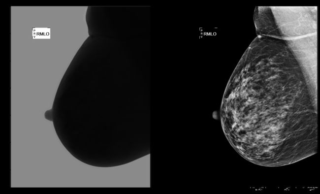
# visualize the two numpy arrays
plt.subplot(1,2,1)
plt.imshow(raw_np, cmap='gray')
plt.title('raw data')
plt.subplot(1,2,2)
plt.imshow(out_np, cmap='gray')
plt.title('gray-level data (target)')
plt.show()
def sitk_show(img, title=None, margin=0.0, dpi=40):
    nda = sitk.GetArrayFromImage(img)
    #spacing = img.GetSpacing()
    figsize = (1 + margin) * nda.shape[0] / dpi, (1 + margin) * nda.shape[1] / dpi
    #extent = (0, nda.shape[1]*spacing[1], nda.shape[0]*spacing[0], 0)
    extent = (0, nda.shape[1], nda.shape[0], 0)
    fig = plt.figure(figsize=figsize, dpi=dpi)
    ax = fig.add_axes([margin, margin, 1 - 2*margin, 1 - 2*margin])

    plt.set_cmap("gray")

    ax.imshow(nda,extent=extent,interpolation=None)

    if title:
        plt.title(title)

    plt.show()
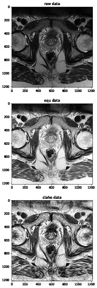
图像预处理技术——CLAHE
- 限制对比度自适应直方图均衡(CLAHE算法)是一种效果较好的均衡算法
- 与普通的自适应直方图均衡相比,CLAHE的 不同地方在于直方图修剪过程,用修剪后的 直方图均衡图像时,图像对比度会更自然。
CLAHE算法步骤
- 图像分块,以块为单位,先计算直方图,然后修剪直方图,最后均衡;
- 遍历、操作各个图像块,进行块间双线性插值;
- 与原图做图层滤色混合操作。(可选)
import cv2
# raw and gray-level data in ITK format
raw = cv2.imread('1.png', 0)
equ = cv2.equalizeHist(raw)  # 应用全局直方图均衡化

clahe = cv2.createCLAHE(clipLimit=100, tileGridSize=(8, 8))  # 自适应均衡化,参数可选
cl1 = clahe.apply(raw)

# visualize the two numpy arrays
plt.subplot(3,1,1)
plt.imshow(raw, cmap='gray')
plt.title('raw data')
plt.subplot(3,1,2)
plt.imshow(equ, cmap='gray')
plt.title('equ data')
plt.subplot(3,1,3)
plt.imshow(cl1, cmap='gray')
plt.title('clahe data')
plt.show()
常用的图像处理
将一张原始图片转换为一张灰度图片,需要实现下面3个主要步骤:
- 对数变换
- 图像强度反转
- 对比度拉伸

对数变换
# logarithmic transformation
# >> YOUR CODE HERE <<<
# The mu and d actually stand for depth and intensitiy in the scan
# It does not have to be incorporated into the calculations
print(raw_np)
mammo_log = np.log(raw_np + 1)
mammo_log = mammo_log *(255/np.max(mammo_log))
print("Lowest value in mammo_log:" + str(np.min(mammo_log)))
print("Highest value in mammo_log:" + str(np.max(mammo_log)))
print(mammo_log)
[[16383 16383 16383 ... 16383 16383 16383]
 [16383 16383 16383 ... 16383 16383 16383]
 [16383 16383 16383 ... 16383 16383 16383]
 ...
 [ 8832  8832  8832 ...  8832  8832  8832]
 [ 8832  8832  8832 ...  8832  8832  8832]
 [ 8832  8832  8832 ...  8832  8832  8832]]
Lowest value in mammo_log:0.0
Highest value in mammo_log:255.0
[[255.     255.     255.     ... 255.     255.     255.    ]
 [255.     255.     255.     ... 255.     255.     255.    ]
 [255.     255.     255.     ... 255.     255.     255.    ]
 ...
 [238.7654 238.7654 238.7654 ... 238.7654 238.7654 238.7654]
 [238.7654 238.7654 238.7654 ... 238.7654 238.7654 238.7654]
 [238.7654 238.7654 238.7654 ... 238.7654 238.7654 238.7654]]
assert(mammo_log is not None),"mammo_log cannot be None"

# visualize the result
plt.imshow(mammo_log, cmap='gray')
plt.title('after logaritmic transformation')
Text(0.5,1,'after logaritmic transformation')
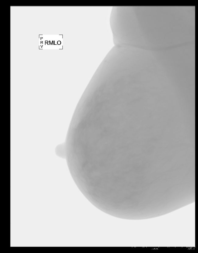
图像强度反转
# intensity inversion
# >> YOUR CODE HERE <<<

# In order to make np.invert work, we have to convert floats to ints
# mammo_inv = np.invert(mammo_log.astype(int))
# numpy invert is a elementwise operation. The TA told us that we should invert the values by ourself.
mammo_inv = (mammo_log-np.max(mammo_log))*-1
print("Lowest value in mammo_inv:" + str(np.min(mammo_inv)))
print("Highest value in mammo_inv:" + str(np.max(mammo_inv)))
Lowest value in mammo_inv:-0.0
Highest value in mammo_inv:255.0
assert(mammo_inv is not None),"mammo_inv cannot be None"

# visualize the result
plt.imshow(mammo_inv, cmap='gray')
plt.title('after intensity inversion')
Text(0.5,1,'after intensity inversion')

对比度拉伸
为了应用对比度拉伸操作,我们首先定义一般的对比度拉伸功能。 输入应至少为:
- 输入信号,
- 窗口范围值p0和pk。
注意:最终结果不应包含大于pk或低于p0的强度值。
# contrast stretching
def contrast_stretching(x, p0, pk, q0=0., qk=255.):
    # >>> YOUR CODE HERE <<<
    x_cs = (x-p0)/(pk-p0)
    x_cs[x_cs<=0] = 0 # Clipping, suggested by TA
    x_cs[x_cs>1]  = 1 # Clipping, suggested by TA
    x_cs = q0 + (qk - q0) * x_cs
    return x_cs
现在我们可以应用对比度拉伸并可视化结果。
# plotting histogram to choose proper boundaries (p0, pk)
hist, bin_edges = np.histogram(mammo_inv, bins=500, range=[75, 110])
plt.bar(bin_edges[:-1], hist, width = 1)
plt.xlim(min(bin_edges), max(bin_edges))
plt.show()

# pick proper values for p0 and pk
p0 = 85
pk = 100

assert(p0 is not None),"p0 cannot be None"
assert(pk is not None),"pk cannot be None"

mammo_cs = contrast_stretching(mammo_inv, p0, pk)
assert(mammo_cs is not None),"mammo_cs can not be None"

# visualize the result
plt.imshow(mammo_cs, cmap='gray')
plt.show()

您会注意到此阶段的结果已经比您开始的原始数据更具可读性。 然而,结果仍然不如乳腺X光片厂商提供的效果好。 为了检查两者的差异,我们将在反转后(对比度拉伸之前),对比度拉伸之后和目标拉伸之后的结果和可视化乳腺X光片厂商处理图的直方图进行比较。
# visualize and compare histograms
plt.subplot(1,3,1)
plt.hist(mammo_inv.flatten(), 100)
plt.title('before contrast stretching')
plt.subplot(1,3,2)
plt.hist(mammo_cs.flatten(), 100)
plt.title('after contrast stretching')
plt.subplot(1,3,3)
plt.hist(out_np.flatten(), 100)
plt.title('target')
plt.show()

答案:通过绘制倒置图像的直方图,我们寻找一般峰值并隔离每个峰值,并将它们用于对比度拉伸的候选参数。 在分离并尝试了三个不同的峰值之后,我们确定了85到100之间的范围,因为它产生了与厂商处理图片的效果。 0和30左右的第一个峰值仅产生前景和背景之间的分离,因此不是我们正在寻找的解决参数。 如果更改这些参数,则只需将要合并的范围限制为对比度拉伸过程。 这些参数的微小变化可能导致具有不同细节水平的不同图像。 因此,直方图是隔离对比度拉伸的参数选择的有用工具。
直方图均衡/匹配
对比度拉伸的步骤可以用直方图均衡来代替。 通过这种方式,我们假设目标图像是已知的,我们将从中学习一些强度值对应函数,称为查找表(LUT)。 LUT是一个表格,其条目对应于输入图像中的所有可能值,并且每个值都映射到输出值,目的是模仿目标图像的强度分布,在我们的案例中是乳腺X光片供应商处理结果。
实现一个函数,该函数将直方图作为输入进行变换,并使用目标直方图并返回LUT。
# function to do histogram matching

def get_histogram_matching_lut(h_input, h_template):
    ''' h_input: histogram to transfrom, h_template: reference'''
    if len(h_input) != len(h_template):
        print('histograms length mismatch!')
        return False

    # >> YOUR CODE HERE <<
    LUT = np.zeros(len(h_input))
    H_input = np.cumsum(h_input) # Cumulative distribution of h_input
    H_template = np.cumsum(h_template) # Cumulative distribution of h_template

    for i in range(len(H_template)):
        input_index = H_input[i]
        new_index = (np.abs(H_template-input_index)).argmin()
        LUT[i] = new_index

    return LUT, H_input, H_template
现在已经实现了函数get_histogram_matching_lut(),你可以执行下一个使用它的单元格,并可视化使用直方图匹配转换的乳腺X光片图像的结果。
# rescale images between [0,1]
out_np = out_np.astype(float)
mammo_inv_norm = (mammo_inv - mammo_inv.flatten().min())/(mammo_inv.flatten().max() - mammo_inv.flatten().min())
mammo_out_norm = (out_np - out_np.flatten().min())/(out_np.flatten().max() - out_np.flatten().min())
n_bins = 4000 # define the number of bins
hist_inv = np.histogram(mammo_inv_norm, bins=np.linspace(0., 1., n_bins+1))
hist_out = np.histogram(mammo_out_norm, bins=np.linspace(0., 1., n_bins+1))
# compute LUT
LUT,H_input,H_template = get_histogram_matching_lut(hist_inv[0], hist_out[0])
assert(LUT is not None),"LUT cannot be None"
assert(H_input is not None),"H_input cannot be None"
assert(H_template is not None),"H_template cannot be None"
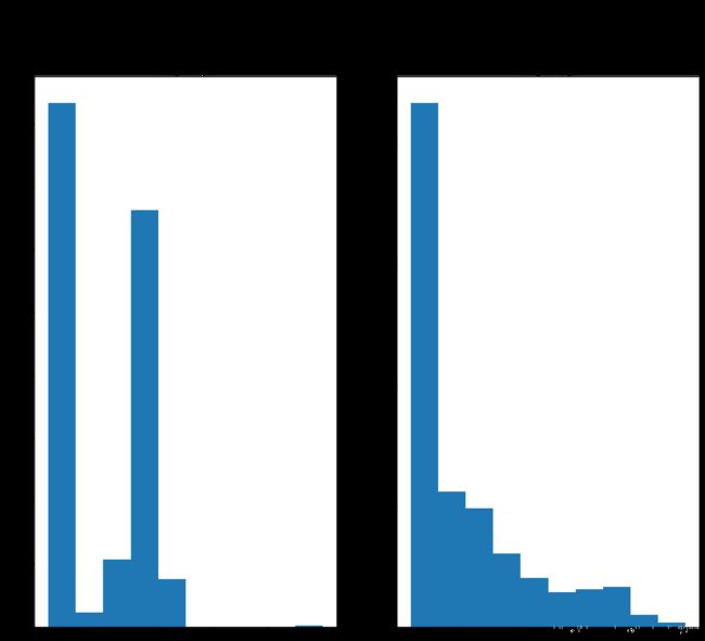
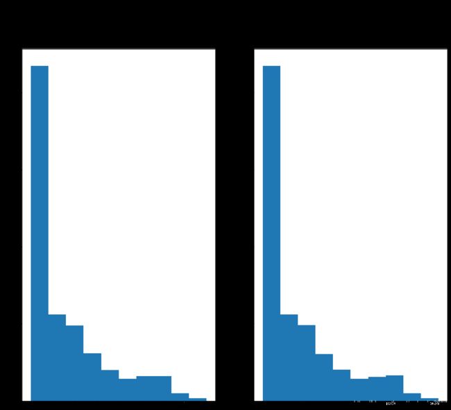
# histograms before matching
plt.suptitle('BEFORE HISTOGRAM MATCHING')
plt.subplot(1,2,1); plt.hist(mammo_inv_norm.flatten())
plt.title('histogram input')
plt.subplot(1,2,2); plt.hist(mammo_out_norm.flatten())
plt.title('histogram target')
plt.show()
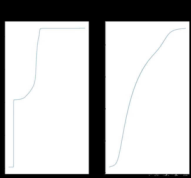
# plot cumulative histogram
plt.suptitle('CUMULATIVE HISTOGRAMS')
plt.subplot(1,2,1); plt.plot(H_input)
plt.title('cumulative histogram input')
plt.subplot(1,2,2); plt.plot(H_template)
plt.title('cumulative histogram target')
plt.show()
# apply histogram matching
mammo_lut = LUT[(mammo_inv_norm * (n_bins-1)).astype(int)]
# visual result
plt.suptitle('VISUAL RESULT')
plt.subplot(1,2,1); plt.imshow(mammo_lut.squeeze(), cmap='gray')
plt.title('converted image')
plt.subplot(1,2,2); plt.imshow(out_np, cmap='gray')
plt.title('target')
plt.show()
# histograms after matching
plt.suptitle('AFTER HISTOGRAM MATCHING')
plt.subplot(1,2,1)
plt.hist(mammo_lut.flatten())
plt.subplot(1,2,2)
plt.hist(out_np.flatten())
plt.show()

Question:
你是如何选择用于进行直方图匹配的分箱数? 结果是否取决于分箱的数量?
从目标直方图中获取总分箱数的大小。 似乎结果实际上并不依赖于分箱的数量,因为转换后的图像不会发生变化(很多)。
病理切片的归一化(直方图匹配)
在上一个练习中,我们实现了直方图匹配功能,并使用它来使给定的乳腺X光片图像适应给定的目标图像。在这种情况下,目标是增强原始乳腺X光片数据中的相关信息,并使其作为灰度图像更利于查看。
相同的技术可以应用于数字病理学领域,但是为了解决不同的问题,图像中的染色剂的可变性。
在病理学中,切割组织样品并用特定染料染色,以增强与诊断相关的一些组织。最常用的染色称为Hematoxylyn和Eosin(H&E),常规用于诊断目的。
H&E的问题在于,在一周的不同日期进行染色时,实验室中的染色变异很大,甚至在同一实验室也是如此。这是因为最终结果很大程度上取决于染料的类型和密度以及组织实际暴露于染色剂的时间。
右边的例子是从公开可用的数据集(https://zenodo.org/record/53169#.WJRAC_krIuU) 中提取的结肠直肠癌组织样本的图像,其中HE染色图像的外观,主要是颜色是不同的。
直方图匹配是一种可以帮助解决这个问题的技术,因为我们可以考虑通过独立处理每个通道来调整每个通道(R,G,B)的颜色分布。
使用数字病理切片图像时,值得注意的是图像大小通常很大。典型的组织病理学图像是千兆像素图像,大约100,000 x 100,000像素。但是,为了简单起见,在此任务中,我们将仅使用5000x5000像素的图块。
加载病历切片的数据
# load data
HE1 = np.asarray(Image.open('./assignment_1/CRC-Prim-HE-05_APPLICATION.tif'))
HE2 = np.asarray(Image.open('./assignment_1/CRC-Prim-HE-10_APPLICATION.tif'))

print(HE1.shape)
print(HE2.shape)

plt.subplot(1,2,1); plt.imshow(HE1); plt.title('HE1')
plt.subplot(1,2,2); plt.imshow(HE2); plt.title('HE2')
(5000, 5000, 3)
(5000, 5000, 3)


Text(0.5,1,'HE2')
染色剂归一化
基于直方图匹配,基于以下定义实现染色剂标准化功能。
def stain_normalization(input_img, target_img, n_bins=100):
    """ Stain normalization based on histogram matching. """

    print("Lowest value in input_img:" + str(np.min(input_img)))
    print("Highest value in input_img:" + str(np.max(input_img)))

    print("Lowest value in target_img:" + str(np.min(target_img)))
    print("Highest value in target_img:" + str(np.max(target_img)))

    normalized_img = np.zeros(input_img.shape)

    input_img = input_img.astype(float) # otherwise we get a complete yellow image
    target_img = target_img.astype(float) # otherwise we get a complete blue image

    # Used resource: https://stackoverflow.com/a/42463602
    # normalize input_img
    input_img_min = input_img.min(axis=(0, 1), keepdims=True)
    input_img_max = input_img.max(axis=(0, 1), keepdims=True)
    input_norm = (input_img - input_img_min)/(input_img_max - input_img_min)

    # normalize target_img
    target_img_min = target_img.min(axis=(0, 1), keepdims=True)
    target_img_max = target_img.max(axis=(0, 1), keepdims=True)
    target_norm = (target_img - target_img_min)/(target_img_max - target_img_min)

    # Go through all three channels
    for i in range(3):
        input_hist = np.histogram(input_norm[:,:,i], bins=np.linspace(0, 1, n_bins + 1))
        target_hist = np.histogram(target_norm[:,:,i], bins=np.linspace(0, 1, n_bins + 1))
        LUT, H_input, H_template = get_histogram_matching_lut(input_hist[0],target_hist[0])
        normalized_img[:,:,i] = LUT[(input_norm[:,:,i] * (n_bins - 1)).astype(int)]

    normalized_img = normalized_img / n_bins

    return normalized_img
现在我们可以使用实现的函数进行染色剂归一化并查看实际结果。
# transform HE1 to match HE2
HE1_norm = stain_normalization(HE1, HE2);
assert(HE1_norm is not None),"HE1_norm can not be None"

plt.subplot(1,3,1)
plt.imshow(HE1); plt.title('HE1 before normalization')
plt.subplot(1,3,2)
plt.imshow(HE1_norm); plt.title('HE1 after normalization')
plt.subplot(1,3,3)
plt.imshow(HE2); plt.title('target')
plt.show()

# transform HE2 to match HE1
HE2_norm = stain_normalization(HE2, HE1);
plt.subplot(1,3,1); plt.imshow(HE2)
plt.title('HE2 before normalization')
plt.subplot(1,3,2); plt.imshow(HE2_norm)
plt.title('HE2 after normalization')
plt.subplot(1,3,3); plt.imshow(HE1)
plt.title('target')
plt.show()
Lowest value in input_img:0
Highest value in input_img:255
Lowest value in target_img:0
Highest value in target_img:255
Lowest value in input_img:0
Highest value in input_img:255
Lowest value in target_img:0
Highest value in target_img:255