Coursera-吴恩达-深度学习-第四门课-卷积神经网络 -week4-编程作业
本文章内容:
Coursera吴恩达深度学习课程,
第四课: 卷积神经网络(Convolutional Neural Networks)
第四周:特殊应用:人脸识别和神经风格转换(Special applications: Face recognition &Neural style transfer)
编程作业
1 - Problem Statement
Neural Style Transfer (NST) is one of the most fun techniques in deep learning. As seen below, it merges two images, namely, a "content" image (C) and a "style" image (S), to create a "generated" image (G). The generated image G combines the "content" of the image C with the "style" of image S.
2 - Transfer Learning
Neural Style Transfer (NST) uses a previously trained convolutional network, and builds on top of that. The idea of using a network trained on a different task and applying it to a new task is called transfer learning.
we will use the VGG network. Specifically, we'll use VGG-19, a 19-layer version of the VGG network. This model has already been trained on the very large ImageNet database, and thus has learned to recognize a variety of low level features (at the earlier layers) and high level features (at the deeper layers).
The model is stored in a python dictionary where each variable name is the key and the corresponding value is a tensor containing that variable's value. To run an image through this network, you just have to feed the image to the model. In TensorFlow, you can do so using the tf.assign function. In particular, you will use the assign function like this:
model["input"].assign(image)
This assigns the image as an input to the model. After this, if you want to access the activations of a particular layer, say layer 4_2 when the network is run on this image, you would run a TensorFlow session on the correct tensor conv4_2, as follows:
sess.run(model["conv4_2"])3 - Neural Style Transfer
We will build the NST algorithm in three steps:
- Build the content cost function Jcontent(C,G)Jcontent(C,G)
- Build the style cost function Jstyle(S,G)Jstyle(S,G)
- Put it together to get J(G)=αJcontent(C,G)+βJstyle(S,G)J(G)=αJcontent(C,G)+βJstyle(S,G
3.1 - Computing the content cost
In our running example, the content image C will be the picture of the Louvre Museum in Paris. Run the code below to see a picture of the Louvre.
3.1.1 - How do you ensure the generated image G matches the content of the image C?
As we saw in lecture, the earlier (shallower) layers of a ConvNet tend to detect lower-level features such as edges and simple textures, and the later (deeper) layers tend to detect higher-level features such as more complex textures as well as object classes.
Instructions: The 3 steps to implement this function are:
- Retrieve dimensions from a_G:
- To retrieve dimensions from a tensor X, use:
X.get_shape().as_list()
- To retrieve dimensions from a tensor X, use:
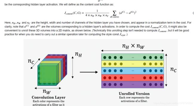
- Unroll a_C and a_G as explained in the picture above
- If you are stuck, take a look at Hint1 and Hint2.
- Compute the content cost:
- If you are stuck, take a look at Hint3, Hint4 and Hint5.
What you should remember:
- The content cost takes a hidden layer activation of the neural network, and measures how different a(C)a(C) and a(G)a(G) are.
- When we minimize the content cost later, this will help make sure GG has similar content as CC.
3.2 - Computing the style cost
For our running example, we will use the following style image:
3.2.1 - Style matrix
The style matrix is also called a "Gram matrix." In linear algebra, the Gram matrix G of a set of vectors (v1,…,vn)(v1,…,vn) is the matrix of dot products, whose entries are Gij=vTivj=np.dot(vi,vj)Gij=viTvj=np.dot(vi,vj). In other words, GijGij compares how similar vivi is to vjvj: If they are highly similar, you would expect them to have a large dot product, and thus for GijGij to be large.
Note that there is an unfortunate collision in the variable names used here. We are following common terminology used in the literature, but GG is used to denote the Style matrix (or Gram matrix) as well as to denote the generated image GG. We will try to make sure which GG we are referring to is always clear from the context.
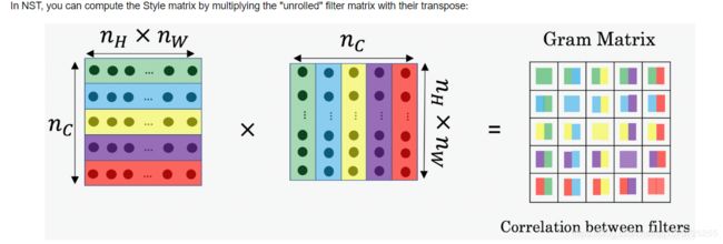
The result is a matrix of dimension (nC,nC)(nC,nC) where nCnC is the number of filters.
The value GijGij measures how similar the activations of filter ii are to the activations of filter jj.
One important part of the gram matrix is that the diagonal elements such as GiiGii also measures how active filter ii is. For example, suppose filter ii is detecting vertical textures in the image. Then GiiGii measures how common vertical textures are in the image as a whole: If GiiGii is large, this means that the image has a lot of vertical texture.
By capturing the prevalence of different types of features (GiiGii), as well as how much different features occur together (GijGij), the Style matrix GG measures the style of an image.
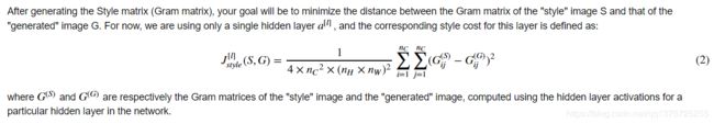
3.2.2 - Style cost
Instructions: The 3 steps to implement this function are:
- Retrieve dimensions from the hidden layer activations a_G:
- To retrieve dimensions from a tensor X, use:
X.get_shape().as_list()
- To retrieve dimensions from a tensor X, use:
- Unroll the hidden layer activations a_S and a_G into 2D matrices, as explained in the picture above.
- You may find Hint1 and Hint2 useful.
- Compute the Style matrix of the images S and G. (Use the function you had previously written.)
- Compute the Style cost:
- You may find Hint3, Hint4 and Hint5 useful.
3.2.3 Style Weights
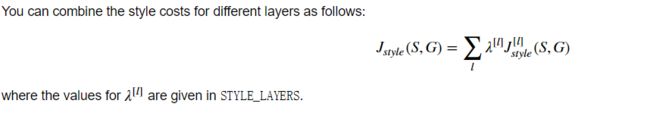
So far you have captured the style from only one layer. We'll get better results if we "merge" style costs from several different layers.
What you should remember:
- The style of an image can be represented using the Gram matrix of a hidden layer's activations. However, we get even better results combining this representation from multiple different layers. This is in contrast to the content representation, where usually using just a single hidden layer is sufficient.
- Minimizing the style cost will cause the image GG to follow the style of the image SS.
3.3 - Defining the total cost to optimize
What you should remember:
- The total cost is a linear combination of the content cost Jcontent(C,G)Jcontent(C,G) and the style cost Jstyle(S,G)Jstyle(S,G)
- αα and ββ are hyperparameters that control the relative weighting between content and style
4 - Solving the optimization problem
Finally, let's put everything together to implement Neural Style Transfer!
Here's what the program will have to do:
- Create an Interactive Session
- Load the content image
- Load the style image
- Randomly initialize the image to be generated
- Load the VGG16 model
- Build the TensorFlow graph:
- Run the content image through the VGG16 model and compute the content cost
- Run the style image through the VGG16 model and compute the style cost
- Compute the total cost
- Define the optimizer and the learning rate
- Initialize the TensorFlow graph and run it for a large number of iterations, updating the generated image at every step.
6 - Conclusion
Great job on completing this assignment! You are now able to use Neural Style Transfer to generate artistic images. This is also your first time building a model in which the optimization algorithm updates the pixel values rather than the neural network's parameters. Deep learning has many different types of models and this is only one of them!
What you should remember:
- Neural Style Transfer is an algorithm that given a content image C and a style image S can generate an artistic image
- It uses representations (hidden layer activations) based on a pretrained ConvNet.
- The content cost function is computed using one hidden layer's activations.
- The style cost function for one layer is computed using the Gram matrix of that layer's activations. The overall style cost function is obtained using several hidden layers.
- Optimizing the total cost function results in synthesizing new images.