In this chapter, we discuss the support vector machine(SVM), an approach for classification that was developed in the computer science community in the 1990s and that has grown in popularity since then. SVMs have been shown to perform well in a variety of settings, and are often considered one of the best “out of the box” classifiers.
The support vector machine is a generalization of a simple and intuitive classifier called the maximal margin classifier , which we introduce in Section 9.1. Though it is elegant and simple, we will see that this classifier unfortunately cannot be applied to most data sets, since it requires that the classes be separable by a linear boundary.
In Section 9.2, we introduce the support vector classifier , an extension of the maximal margin classifier that can be applied in a broader range of cases.
Section 9.3 introduces the support vector machine , which is a further extension of the support vector classifier in order to accommodate non-linear class boundaries.
Support vector machines are intended for the binary classification setting in which there are two classes; in Section 9.4 we discuss extensions of support vector machines to the case of more than two classes.
In Section 9.5 we discuss the close connections between support vector machines and other statistical methods such as logistic regression.
Maximal Margin Classifier
In this section, we define a hyperplane and introduce the concept of an optimal separating hyperplane.
What Is a Hyperplane?
In a p-dimensional space, a hyperplane is a flat affine subspace of dimension p−1.
For instance, in two dimensions, a hyperplane is a flat one-dimensional subspace—in other words, a line.
In three dimensions, a hyperplane is a flat two-dimensional subspace—that is, a plane.
In p >3 dimensions, it can be hard to visualize a hyperplane, but the notion of a
(p −1)-dimensional flat subspace still applies.
The mathematical definition of a hyperplane is quite simple. In two dimensions, a hyperplane is defined by the equation:
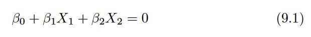
for parameters β0, β1, andβ2. When we say that (9.1) “defines” the hyperplane,we mean that any X= (X1,X2)T for which (9.1) holds is a point on the hyperplane.Note that (9.1) is simply the equation of a line, since indeed in two dimensions a hyperplane is a line.
Equation 9.1 can be easily extended to the p-dimensional setting:
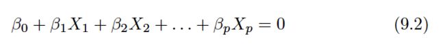
defines a p-dimensional hyperplane, again in the sense that if a point X= (X1,X2, . . . , Xp)T in p-dimensional space (i.e. a vector of lengthp) satisfies (9.2), then X lies on the hyperplane.
Now, suppose that X does not satisfy (9.2); rather,
Then this tells us that X lies to one side of the hyperplane. On the other hand, if:

then X lies on the other side of the hyperplane.
So we can think of the hyperplane as dividing p-dimensional space into two halves. One can easily determine on which side of the hyperplane a point lies by simply calculating the sign of the left hand side of (9.2). A hyperplane in two dimensional space is shown in Figure 9.1.

Classification Using a Separating Hyperplane
Now suppose that we have a n*p data matrix X that consist of n training observations in p-dimensional space,
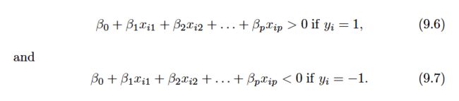
and that these observations fall into two classes—that is,y1, . . . , yn ∈ {− 1,1} where − 1 represents one class and 1 the other class.
We also have a test observation, a p-vector of observed features x=(x1,...,xp).
We have seen a number of approaches for this task, such as linear discriminant analysis and logistic regression in Chapter 4, and classification trees, bagging, and boosting in Chapter 8. We will now see a new approach that is based upon the concept of a separating hyperplane .
The Maximal Margin Classifier
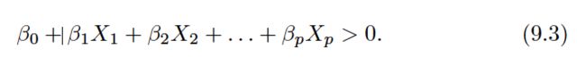
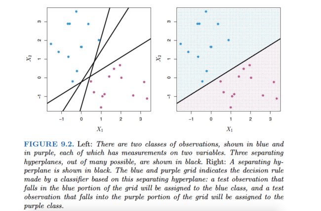
In order to construct a classifier based upon a separating hyperplane, we must have a reasonable way to decide which of the infinite possible separating hyperplanes to use.
A natural choice is the maximal margin hyperplane(also known as the optimal separating hyperplane),which is the separating hyperplane that is farthest from the training observations. That is, we can compute the (perpendicular) distance from each training observation to a given separating hyperplane;the smallest such distance is the minimal distance from the observations to the hyperplane,and is known as the margin .The maximal margin hyperplane is the separating hyperplane for which the margin is largest—that is, it is the hyperplane that has the farthest minimum distance to the training observations.We can then classify a test observation based on which side of the maximal margin hyperplane it lies. This is known as the maximal margin classifier .
We hope that a classifier that has a large margin on the training data will also have a large margin on the test data,and hence will classify the test observations correctly. Although the maximal margin classifier is often successful, it can also lead to overfitting when p is large.
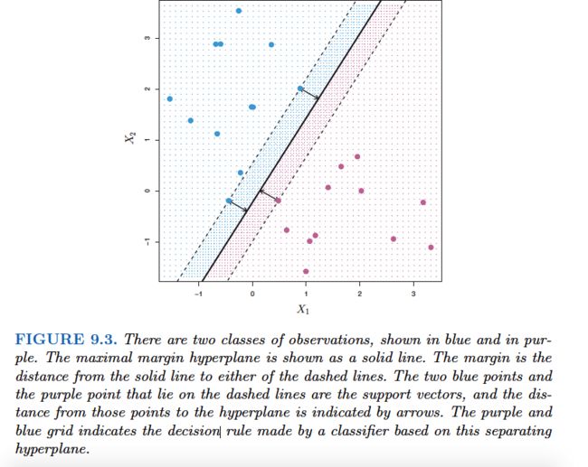
Examining Figure 9.3, we see that three training observations are equidistant from the maximal margin hyperplane and lie along the dashed lines indicating the width of the margin.These three observations are known as support vectors, since they are vectors in p-dimensional space and they “support” the maximal margin hyperplane in the sense that if these points were moved slightly then the maximal margin hyperplane would move as well.Interestingly, the maximal margin hyperplane depends directly on the support vectors,but not on the other observations:a movement to any of the other observations would not affect the separating hyperplane,provided that the observation’s movement does not cause it to cross the boundary set by the margin.The fact that the maximal margin hyperplane depends directly on only a small subset of the observations is an important property that will arise later in this chapter when we discuss the support vector classifier and support vector machines.
Construction of the Maximal Margin Classifier
We now consider the task of constructing the maximal margin hyperplane based on a set of n training observations x1, . . . , xn∈Rp and associated class labels y1, . . . , yn ∈ {− 1,1} . Briefly, the maximal margin hyperplane is the solution to the optimization problem:
M represents the margin of our hyperplane, and the optimization problem choosesβ0, β1, . . . , βp to maximize M.This is exactly the definition of the maximal margin hyperplane! The problem (9.9)–(9.11) can be solved efficiently, but details of this optimization are outside of the scope of this book.
The Non-separable Case
The maximal margin classifier is a very natural way to perform classification, if a separating hyperplane exists . However, as we have hinted, in many cases no separating hyperplane exists,and so there is no maximal margin classifier. In this case, the optimization problem (9.9)–(9.11) has no solution with M > 0.
An example is shown in Figure 9.4. In this case, we cannot exactly separate the two classes. However, as we will see in the next section, we can extend the concept of a separating hyperplane in order to develop a hyperplane that almost separates the classes, using a so-called soft margin . The generalization of the maximal margin classifier to the non-separable case is known as the support vector classifier .

Support Vector Classifiers
Overview of the Support Vector Classifier
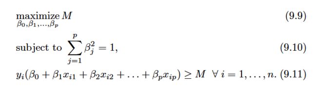
In Figure 9.4, we see that observations that belong to two classes are not necessarily separable by a hyperplane. In fact, even if a separating hyperplane does exist, then there are instances in which a classifier based on a separating hyperplane might not be desirable. A classifier based on a separating hyperplane will necessarily perfectly classify all of the training observations; this can lead to sensitivity to individual observations. An example is shown in Figure 9.5.The addition of a single observation in the right-hand panel of Figure 9.5 leads to a dramatic change in the maximal margin hyperplane.The resulting maximal margin hyperplane is not satisfactory—for one thing, it has only a tiny margin. This is problematic because as discussed previously, the distance of an observation from the hyperplane can be seen as a measure of our confidence that the observation was correctly classified. Moreover, the fact that the maximal margin hyperplane is extremely sensitive to a change in a single observation suggests that it may have overfit the training data.
In this case, we might be willing to consider a classifier based on a hyperplane that does not perfectly separate the two classes, in the interest of
• Greater robustness to individual observations, and
• Better classification of most of the training observations.
That is, it could be worthwhile to misclassify a few training observations in order to do a better job in classifying the remaining observations.
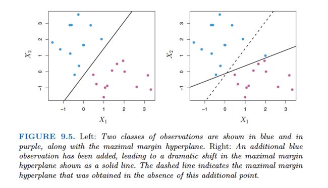
The support vector classifier , sometimes called a soft margin classifier ,does exactly this. Rather than seeking the largest possible margin so that every observation is not only on the correct side of the hyperplane but also on the correct side of the margin, we instead allow some observations to be on the incorrect side of the margin, or even the incorrect side of the hyperplane. (The margin is soft because it can be violated by some of the training observations.) An example is shown in the left-hand panel of Figure 9.6. Most of the observations are on the correct side of the margin. However, a small subset of the observations are on the wrong side of the margin.
An observation can be not only on the wrong side of the margin, but also on the wrong side of the hyperplane. In fact, when there is no separating hyperplane, such a situation is inevitable. Observations on the wrong side of the hyperplane correspond to training observations that are misclassified by the support vector classifier. The right-hand panel of Figure 9.6 illustrates such a scenario.
Details of the Support Vector Classifier
The support vector classifier classifies a test observation depending on which side of a hyperplane it lies. The hyperplane is chosen to correctly separate most of the training observations into the two classes, but may misclassify a few observations. It is the solution to the optimization problem:

where C is a nonnegative tuning parameter. As in (9.11), M is the width of the margin; we seek to make this quantity as large as possible. In (9.14),ei are slack variables that allow individual observations to be on the wrong side of the margin or the hyperplane; we will explain them in greater detail momentarily.
Once we have solved (9.12)–(9.15), we classify a test observation x∗ as before, by simply determining on which side of the hyperplane it lies.
The problem (9.12)–(9.15) seems complex, but insight into its behavior can be made through a series of simple observations presented below.First of all, the slack variable ei tells us where the ith observation is located,relative to the hyperplane and relative to the margin.If ei= 0 then the ith observation is on the correct side of the margin, as we saw in Section 9.1.4.If ei>0 then the ith observation is on the wrong side of the margin, and we say that the ith observation has violated the margin. If ei>1 then it is on the wrong side of the hyperplane.
We now consider the role of the tuning parameter C. In (9.14),C bounds the sum of the ei’s, and so it determines the number and severity of the violations to the margin (and to the hyperplane) that we will tolerate. We can think of C as a budget for the amount that the margin can be violated by the n observations. If C= 0 then there is no budget for violations to the margin, and it must be the case that e1=. . .=en= 0, in which case (9.12)–(9.15) simply amounts to the maximal margin hyperplane optimization problem (9.9)–(9.11). (Of course, a maximal margin hyperplane exists only if the two classes are separable.)
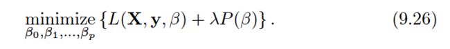
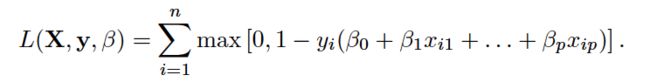
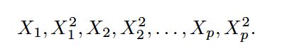
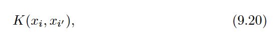
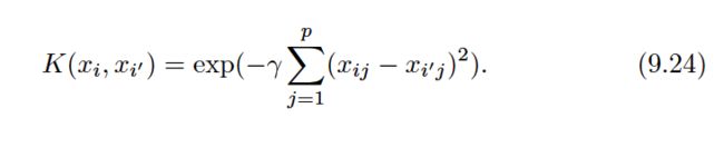
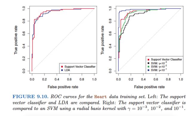
For C >0 no more than C observations can be on the wrong side of the hyperplane, because if an observation is on the wrong side of the hyperplane the ei>1, and (9.14) requires that ei+...+en In practice, C is treated as a tuning parameter that is generally chosen via cross-validation. As with the tuning parameters that we have seen throughout this book, C controls the bias-variance trade-off of the statistical learning technique. When C is small, we seek narrow margins that are rarely violated; this amounts to a classifier that is highly fit to the data, which may have low bias but high variance. On the other hand, when C is larger, the margin is wider and we allow more violations to it; this amounts to fitting the data less hard and obtaining a classifier that is potentially more biased but may have lower variance. The optimization problem (9.12)–(9.15) has a very interesting property: it turns out that only observations that either lie on the margin or that violate the margin will affect the hyperplane, and hence the classifier obtained. In other words, an observation that lies strictly on the correct side of the margin does not affect the support vector classifier! Changing the position of that observation would not change the classifier at all, provided that its position remains on the correct side of the margin. Observations that lie directly on the margin, or on the wrong side of the margin for their class, are known as support vectors . These observations do affect the support vector classifier. The fact that only support vectors affect the classifier is in line with our previous assertion that C controls the bias-variance trade-off of the support vector classifier. When the tuning parameter C is large, then the margin is wide, many observations violate the margin, and so there are many support vectors. In this case, many observations are involved in determining the hyperplane. The top left panel in Figure 9.7 illustrates this setting: this classifier has low variance (since many observations are support vectors) but potentially high bias. In contrast, if C is small, then there will be fewer support vectors and hence the resulting classifier will have low bias but high variance. The bottom right panel in Figure 9.7 illustrates this setting, with only eight support vectors. The fact that the support vector classifier’s decision rule is based only on a potentially small subset of the training observations (the support vectors) means that it is quite robust to the behavior of observations that are far away from the hyperplane. This property is distinct from some of the other classification methods that we have seen in preceding chapters, such as linear discriminant analysis. Recall that the LDA classification rule depends on the mean of all of the observations within each class, as well as the within-class covariance matrix computed using all of the observations. In contrast, logistic regression, unlike LDA, has very low sensitivity to observations far from the decision boundary. In fact we will see in Section 9.5 that the support vector classifier and logistic regression are closely related. We first discuss a general mechanism for converting a linear classifier into one that produces non-linear decision boundaries. We then introduce the support vector machine, which does this in an automatic way. The support vector classifier is a natural approach for classification in the two-class setting, if the boundary between the two classes is linear. However, in practice we are sometimes faced with non-linear class boundaries. For instance, consider the data in the left-hand panel of Figure 9.8. It is clear that a support vector classifier or any linear classifier will perform poorly here. Indeed, the support vector classifier shown in the right-hand panel of Figure 9.8 is useless here. In Chapter 7, we are faced with an analogous situation. We see there that the performance of linear regression can suffer when there is a nonlinear relationship between the predictors and the outcome. In that case, we consider enlarging the feature space using functions of the predictors,such as quadratic and cubic terms, in order to address this non-linearity. In the case of the support vector classifier, we could address the problem of possibly non-linear boundaries between classes in a similar way, by enlarging the feature space using quadratic, cubic, and even higher-order polynomial functions of the predictors. For instance, rather than fitting a support vector classifier using p features: we could instead fit a support vector classifier using 2p features Then: Why does this lead to a non-linear decision boundary? In the enlarged feature space, the decision boundary that results from (9.16) is in fact linear. But in the original feature space, the decision boundary is of the form q(x) = 0, where q is a quadratic polynomial, and its solutions are generally non-linear. Alternatively, other functions of the predictors could be considered rather than polynomials. It is not hard to see that there are many possible ways to enlarge the feature space, and that unless we are careful, we could end up with a huge number of features. Then computations would become unmanageable. The support vector machine, which we present next, allows us to enlarge the feature space used by the support vector classifier in a way that leads to efficient computations. The support vector machine(SVM) is an extension of the support vector classifier that results from enlarging the feature space in a specific way, using kernels . We will now discuss this extension, the details of which are somewhat complex and beyond the scope of this book. However, the main idea is described in Section 9.3.1: we may want to enlarge our feature space in order to accommodate a non-linear boundary between the classes. The kernel approach that we describe here is simply an efficient computational approach for enacting this idea. We have not discussed exactly how the support vector classifier is compute because the details become somewhat technical. However, it turns out that the solution to the support vector classifier problem (9.12)–(9.15) involves only the inner products of the observations (as opposed to the observations themselves). The inner product of two r-vectors a and b is defined as <a, b> Thus the inner product of two observations xi,xi’ is given by: It can be shown that •The linear support vector classifier can be represented as where there are n parameters αi, i= 1, . . . , n , one per training observation. •To estimate the parameters α1, . . . , αn and β0, all we need are n(n-1)/2 inner products Notice that in (9.18), in order to evaluate the function f(x), we need to compute the inner product between the new point x and each of the training points xi. However, it turns out that αi is nonzero only for the support vectors in the solution—that is, if a training observation is not a support vector, then its αi equals zero. So if S is the collection of indices of these support points, we can rewrite any solution function of the form (9.18) as: which typically involves far fewer terms than in (9.18). To summarize, in representing the linear classifier f(x), and in computing its coefficients, all we need are inner products. Now suppose that every time the inner product (9.17) appears in the representation (9.18), or in a calculation of the solution for the support vector classifier, we replace it with a generalization of the inner product of the form: where K is some function that we will refer to as a kernel . A kernel is a function that quantifies the similarity of two observations. For instance, we could simply take which would just give us back the support vector classifier. Equation 9.21 is known as a linear kernel because the support vector classifier is linear in the features;the linear kernel essentially quantifies the similarity of a pair of observations using Pearson (standard) correlation.But one could instead choose another form for (9.20). For instance: This is known as a polynomial kernel of degree d, where d is a positive integer. Using such a kernel with d >1, instead of the standard linear kernel(9.21),in the support vector classifier algorithm leads to a much more flexible decision boundary. It essentially amounts to fitting a support vector classifier in a higher-dimensional space involving polynomials of degree d, rather than in the original feature space. When the support vector classifier is combined with a non-linear kernel such as (9.22), the resulting classifier is known as a support vector machine. Note that in this case the (non-linear) function has the form The left-hand panel of Figure 9.9 shows an example of an SVM with a polynomial kernel applied to the non-linear data from Figure 9.8. The fit is a substantial improvement over the linear support vector classifier. When d= 1, then the SVM reduces to the support vector classifier seen earlier in this chapter. The polynomial kernel shown in (9.22) is one example of a possible non-linear kernel, but alternatives abound. Another popular choice is the radial kernel , which takes the form: What is the advantage of using a kernel rather than simply enlarging the feature space using functions of the original features, as in (9.16)? One advantage is computational,This can be done without explicitly working in the enlarged feature space.This is important because in many applications of SVMs, the enlarged feature space is so large that computations are intractable. For some kernels, such as the radial kernel (9.24), the feature space is implicit and infinite-dimensional, so we could never do the computations there anyway! So far, our discussion has been limited to the case of binary classification: that is, classification in the two-class setting. How can we extend SVMs to the more general case where we have some arbitrary number of classes? It turns out that the concept of separating hyperplanes upon which SVMs are based does not lend itself naturally to more than two classes. Though a number of proposals for extending SVMs to the K-class case have been made, the two most popular are the one-versus-one and one-versus-all approaches. We briefly discuss those two approaches here. Suppose that we would like to perform classification using SVMs, and there are K >2 classes. A one-versus-one or all-pairs approach constructs k(k-1)/2 SVMs,each of which compares a pair of classes. For example, one such SVM might compare the kth class, coded as +1, to the kth class, coded as −1. We classify a test observation using each of the k(k-1)/2 classifiers, and we tally the number of times that the test observation is assigned to each of the K classes. The final classification is performed by assigning the test observation to the class to which it was most frequently assigned in these pairwise classifications. We fit K SVMs, each time comparing one of all the K classes to the remaining K −1 classes.Let x denote a test observation. We assign the observation to the class for which β0k+β1kx1+β2kx2+. . .+βpkxp is largest, as this amounts to a high level of confidence that the test observation belongs to the kth class rather than to any of the other classes. When SVMs were first introduced in the mid-1990s, they made quite a splash in the statistical and machine learning communities. This was due in part to their good performance, good marketing, and also to the fact that the underlying approach seemed both novel and mysterious. The idea of finding a hyperplane that separates the data as well as possible, while allowing some violations to this separation, seemed distinctly different from classical approaches for classification, such as logistic regression and linear discriminant analysis. Moreover, the idea of using a kernel to expand the feature space in order to accommodate non-linear class boundaries appeared to be a unique and valuable characteristic. However, since that time, deep connections between SVMs and other more classical statistical methods have emerged. It turns out that one can rewrite the criterion (9.12)–(9.15) for fitting the support vector classifier f(X) =β0+β1X1+. . .+βpXp as where λ is a nonnegative tuning parameter.When λ is large then β1, . . . , βp are small, more violations to the margin are tolerated,and a low-variance but high-bias classifier will result.When λ is small then few violations to the margin will occur; this amounts to a high-variance but low-bias classifier. Thus, a small value of λ in (9.25) amounts to a small value of C in (9.15). Notes that term in (9.25) is the ridge penalty term from Section 6.2.1, and plays a similar role in controlling the bias-variance trade-off for the support vector classifier. Now (9.25) takes the “Loss + Penalty” form that we have seen repeatedly throughout this book: This is known as hinge loss , and is depicted in Figure 9.12. However, it turns out that the hinge loss function is closely related to the loss function used in logistic regression, also shown in Figure 9.12. An interesting characteristic of the support vector classifier is that only support vectors play a role in the classifier obtained; observations on the correct side of the margin do not affect it.This is due to the fact that the loss function shown in Figure 9.12 is exactly zero for observations for which yi(β0+β1xi1+. . .+βpxip) ≥1;these correspond to observations that are on the correct side of the margin.In contrast, the loss function for logistic regression shown in Figure 9.12 is not exactly zero anywhere. But it is very small for observations that are far from the decision boundary. Due to the similarities between their loss functions, logistic regression and the support vector classifier often give very similar results. When the classes are well separated, SVMs tend to behave better than logistic regression; in more overlapping regimes, logistic regression is often preferred. When the support vector classifier and SVM were first introduced, it was thought that the tuning parameter C in (9.15) was an unimportant “nuisance” parameter that could be set to some default value, like 1. However, the “Loss + Penalty” formulation (9.25) for the support vector classifier indicates that this is not the case. The choice of tuning parameter is very important and determines the extent to which the model underfits or overfits the data, as illustrated, for example, in Figure 9.7. We have established that the support vector classifier is closely related to logistic regression and other preexisting statistical methods. Is the SVM unique in its use of kernels to enlarge the feature space to accommodate non-linear class boundaries? The answer to this question is “no”. We could just as well perform logistic regression or many of the other classification methods seen in this book using non-linear kernels; this is closely related to some of the non-linear approaches seen in Chapter 7. However, for historical reasons, the use of non-linear kernels is much more widespread in the context of SVMs than in the context of logistic regression or other methods.(kernel技巧在很多统计学习中都可以使用) Though we have not addressed it here, there is in fact an extension of the SVM for regression (i.e. for a quantitative rather than a qualitative response), called support vector regression. In Chapter 3, we saw that least squares regression seeks coefficients β0, β1, . . . , βp such that the sum of squared residuals is as small as possible. Support vector regression instead seeks coefficients that minimize a different type of loss, where only residuals larger in absolute value than some positive constant contribute to the loss function. This is an extension of the margin used in support vector classifiers to the regression setting.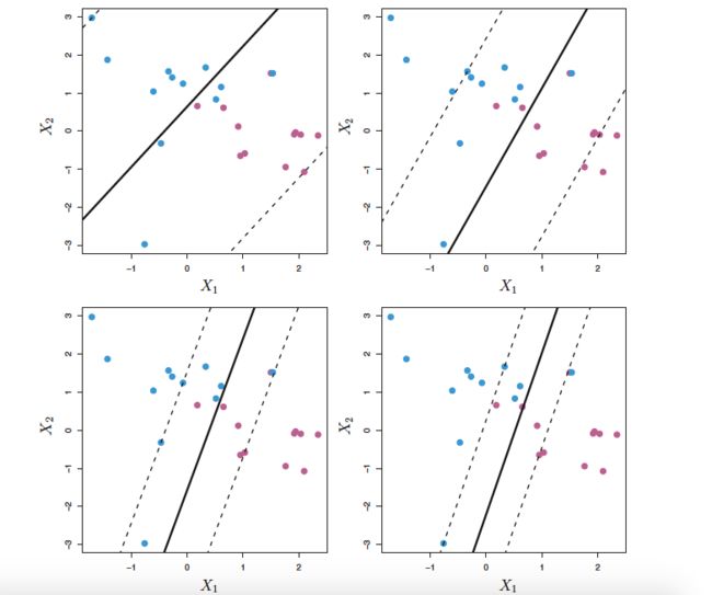

Support Vector Machines
Classification with Non-linear Decision Boundaries


The Support Vector Machine


SVMs with More than Two Classes
One-Versus-One Classification
One-Versus-All Classification
Relationship to Logistic Regression