So far in this book, we have mostly focused on linear models. Linear models are relatively simple to describe and implement, and have advantages over other approaches in terms of interpretation and inference.
In Chapter 6 we see that we can improve upon least squares using ridge regression, the lasso, principal components regression, and other techniques. In that setting, the improvement is obtained by reducing the complexity of the linear model, and hence the variance of the estimates. But we are still using a linear model, which can only be improved so far!
In this chapter we relax the linearity assumption while still attempting to maintain as much interpretability as possible.We do this by examining very simple extensions of linear models like polynomial regression and step functions, as well as more sophisticated approaches such as splines, local regression, and generalized additive models.
• Polynomial regression extends the linear model by adding extra predictors, obtained by raising each of the original predictors to a power.For example, a cubic regression uses three variables,X,X2, and X3, as predictors. This approach provides a simple way to provide a nonlinear fit to data.
• Step functions cut the range of a variable into K distinct regions in order to produce a qualitative variable. This has the effect of fitting a piecewise constant function.
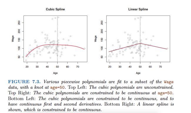
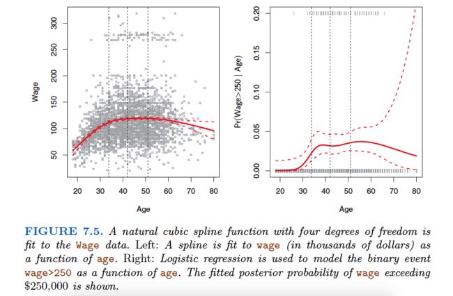
• Regression splines are more flexible than polynomials and step functions, and in fact are an extension of the two. They involve dividing the range of X into K distinct regions. Within each region, a polynomial function is fit to the data. However, these polynomials are constrained so that they join smoothly at the region boundaries, or knots. Provided that the interval is divided into enough regions, this can produce an extremely flexible fit.
• Smoothing splines are similar to regression splines, but arise in a slightly different situation. Smoothing splines result from minimizing a residual sum of squares criterion subject to a smoothness penalty.
• Local regression is similar to splines, but differs in an important way. The regions are allowed to overlap, and indeed they do so in a very smooth way.
• Generalized additive models allow us to extend the methods above to deal with multiple predictors.
Polynomial Regression
Generally speaking, it is unusual to use d greater than 3 or 4 because for large values of d , the polynomial curve can become overly flexible and can take on some very strange shapes.
Step Functions
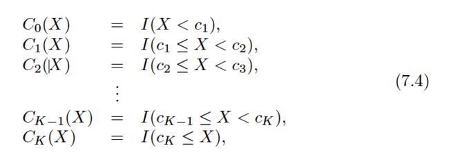
Using polynomial functions of the features as predictors in a linear model imposes a global structure on the non-linear function of X. We can instead use step functions in order to avoid imposing such a global structure. Here we break the range of X into bins , and fit a different constant in each bin. This amounts to converting a continuous variable into an ordered categorical variable .
These are sometimes called dummy variables. Notice that for any value of X,C0(X)+C1(X)+. . .+CK(X) = 1, since X must be in exactly one of the K+ 1 intervals.
Basis Functions
Polynomial and piecewise-constant regression models are in fact special cases of a basis function approach.
Note that the basis functions b1(xi), b2(xi), . . . , bK(xi) are fixed and known.In other words, we choose the functions ahead of time.
For polynomial regression, the basis functions are bj(xi) =xji, and for piecewise constant functions they are bj(xi) = I(cj≤xi< cj+1).
We can think of as a standard linear model with predictors b1(xi), b2(xi), . . . , bK(xi).
Regression Splines
Piecewise Polynomials
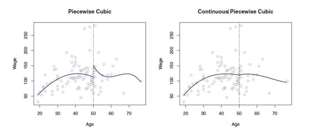
Instead of fitting a high-degree polynomial over the entire range of X, piecewise polynomial regression involves fitting separate low-degree polynomials over different regions of X. For example, a piecewise cubic polynomial works by fitting a cubic regression model of the form:
where the coefficients β0,β1,β2, and β3 differ in different parts of the range of X. The points where the coefficients change are called knots .
Constraints and Splines
The Spline Basis Representation
A truncated power basis function is defined as:
where ξ is the knot.
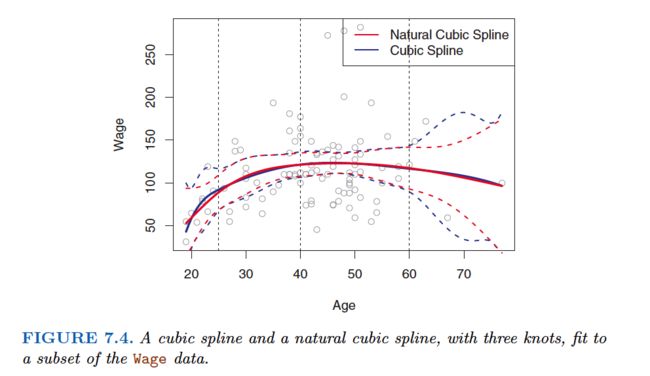
In other words, in order to fit a cubic spline to a data set with K knots, we perform least squares regression with an intercept and 3+K predictors, of the form X,X2,X3, h (X, ξ1), h (X, ξ2), . . . , h (X, ξK), where ξ1, . . . , ξKare the knots. This amounts to estimating a total of K+ 4 regression coefficients; for this reason, fitting a cubic spline with K knots uses K +4 degrees of freedom.
Choosing the Number and Locations of the Knots
One way to do this is to specify the desired degrees of freedom, and then have the software automatically place the corresponding number of knots at uniform quantiles of the data.
How many knots should we use, or equivalently how many degrees of freedom should our spline contain? One option is to try out different numbers of knots and see which produces the best looking curve.
A somewhat more objective approach is to use cross-validation.
Comparison to Polynomial Regression
Regression splines often give superior results to polynomial regression.This is because unlike polynomials, which must use a high degree to produce flexible fits, splines introduce flexibility by increasing the number of knots but keeping the degree fixed.
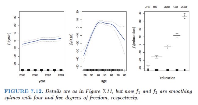
Smoothing Splines
In the last section we discussed regression splines, which we create by specifying a set of knots, producing a sequence of basis functions, and then using least squares to estimate the spline coefficients. We now introduce a somewhat different approach that also produces a spline.
What we really want is a function g that makes RSS small, but that is also smooth .
How might we ensure that gis smooth? There are a number of ways to do this. A natural approach is to find the function g that minimizes:
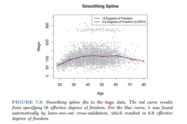
where λ is a nonnegative tuning parameter.The function g that minimizes (7.11) is known as a smoothing spline .
Equation 7.11 takes the “Loss+Penalty” formulation that we encounter in the context of ridge regression and the lasso in Chapter 6.
a loss function that encourages g to fit the data well,and the penalty term that penalizes the variability in g.
Choosing the Smoothing Parameter λ
It is possible to show that as λ increases from 0 to ∞, the effective degrees of freedom, which we write dfλ, decrease from n to 2.
Local Regression
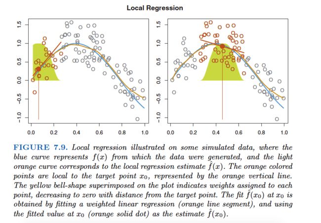
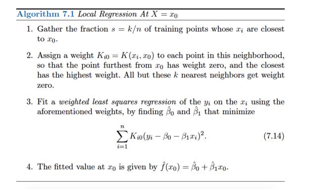
Local regression is a different approach for fitting flexible non-linear functions, which involves computing the fit at a target point x0 using only the nearby training observations.
Local regression is sometimes referred to as a memory-based procedure, because like nearest-neighbors, we need all the training data each time we wish to compute a prediction.
Generalized Additive Models
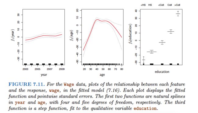
Generalized additive models(GAMs) provide a general framework for extending a standard linear model by allowing non-linear functions of each of the variables, while maintaining additivity.
Just like linear models, GAMs can be applied with both quantitative and qualitative responses.
GAMs for Regression Problems
This is an example of a GAM. It is called an additive model because we calculate a separate fj for each Xj, and then add together all of their contributions.
Pros and Cons of GAMs
GAMs allow us to fit a non-linear fj to each Xj, so that we can automatically model non-linear relationships that standard linear regression will miss. This means that we do not need to manually try out many different transformations on each variable individually.
The non-linear fits can potentially make more accurate predictions for the response Y .
Because the model is additive, we can still examine the effect of each Xj on Y individually while holding all of the other variables fixed. Hence if we are interested in inference, GAMs provide a useful representation.
The smoothness of the function fj for the variable Xj can be summarized via degrees of freedom.
The main limitation of GAMs is that the model is restricted to be additive. With many variables, important interactions can be missed. However, as with linear regression, we can manually add interaction terms to the GAM model by including additional predictors of the form Xj°øXk. In addition we can add low-dimensional interaction functions of the form fjk(Xj,Xk) into the model; such terms can be fit using two-dimensional smoothers such as local regression, or two-dimensional splines (not covered here).
GAMs for Classification Problems
Recall the logistic regression model:
Equation 7.18 is a logistic regression GAM.


