实施DMCplus的第一步是辨识过程动态模型。通过给工厂变量扰动,收集第一手数据,获得工厂模型。运用DMCplus多变量控制软件对工厂数据进行分析。分析得到包含所有显著耦合变量间相互关系的多变量动态模型。
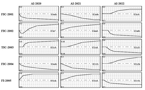
下图显示了一个复杂精馏塔模型。每一格代表对应自变量在0时刻作一阶跃变化,而其它自变量保持恒定时因变量响应(开环阶跃响应)。
简单地说,每条曲线表示自变量变化对对应因变量的影响情况。在后面部分我们将对模型进行进一步说明。
图4:复杂精馏塔模型
得到过程动态模型后,模型将被用于生成和预测过程中CV的未来动态。
模型是基于自变量历史值变化数据计算出预测值的。鉴于所有这些变化会对系统产生持续影响,我们近似认为自变量改变起至一个稳态时间为需要考虑的。变化起一个稳态时间后就不需要考虑,因为它们已经不再影响系统。
由于模型曲线代表了自变量变化对因变量地影响,这些自变量变化可应用于生成模型每一因变量的未来预测值。模型能计算当前时刻一个稳态时间内的预测值。控制器每次执行时会更新因变量预测值,并调和当前预测与实际因变量测量值以消除模型失配的影响。
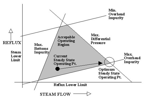
图5:最佳稳态计算参考要素
DMCplus算法下一步是按上图所示计算所有MV和CV的最优稳态目标。计算由稳态线性规划(LP)或稳态二次规划(QP)实现。
计算的输入包括MV(操作变量)当前值和操作限制、CV(被控变量)稳态预测值、产品价值经济信息、原材料和公用工程成本。
操作界限定义了一个可接受的操作区域。MV当前值和CV预测稳态值定义了假设MVs没有移动时预测的稳态工作点。这一点在或不在可接受操作区域内都有可能。
稳态求解器(LP或QP)计算出每个MV的稳态移动,组合后系统给出一个可接受工作区域内的稳态操作点。并且从经济角度看此操作点是最优的。需要注意的是这一最佳稳态操作点始终在上述几个限制下。
下图显示了一包含2个MV(操作变量),3个CV(被控变量)系统例子。
图6:具有2个MV和3个CV系统的操作区域
MVs是回流流量.SP和再沸器蒸汽流量.SP。CVs是塔顶出料杂质,塔釜出料杂质和塔压差。上述五个变量限制下的操作区域为可接受操作区域。
在这个例子中,当前稳态操作点在区域内,尽管不总是这样。同时,当前稳态操作点与当前操作点是不同的;它是系统预测未来没有控制作用的作用点。
知道当前稳态操作点、五个变量限制,和经济信息,就能够确定最佳稳态工作点。该点指定所有MVs和CVs最优稳态目标。
DMCplus算法最后一步是开发MVs控制动作的详细计划以使CVs预测未来性能与期望未来性能误差最小化。CVs期望未来性能是它们的稳态目标,由稳态求解器计算。
CVs稳态目标通常都是CVs的设定点。为了动态驱动CVs到目标值,控制器计算出未来MV一系列动作,一直到未来一半稳态时间左右。这将使控制器推迟控制动作,有利于解决多变量控制问题中一个MV动作对其它MVs的影响。
当所有计算出的MV移动被加入后,MV的值必须等于线性规划中MV稳态目标值。如果所有的MVs达到稳态目标,CVs也将达到稳态目标。
附原文:
The first step in implementing DMCplus is to model the dynamics of the process. The plant model is obtained by first collecting plant data whileperturbing the plant. This plant data is analyzed using DMCplus MultivariableControl software. The result of this analysis is a dynamic, multivariable modelof the process that contains all significant interactions between variables.
Thefigure below shows the model for the Complex Fractionator. Each box representsthe response in time of the dependent variable to a step change at time zero ofthe corresponding independent variable, while all other independent variablesare held constant (open loop step responses).
In simple terms, each curve represents the effect of a change in an independent variable on that dependent variable. The model will be described inmore detail in a later section.
Once the dynamic model has been obtained, this model is used to form and maintain a prediction of future behavior of the controlled variables in the process.
This prediction is maintained by using the past history of changes in the independent variables. All independent variable changes up to one steady-state time into the past are considered, since all of these changes still have an effect on the system. Changes that occurred more than one steady-state time into the past need not be considered, since they no longer affect the system.
Since the model curves represent the effects of independent variable changes on dependent variables, these independent variable changes can be applied to the model to generate a future prediction for each dependent variable. These predictions extend from the current time out to one steady-state time into the future. These dependent variable predictions are updated at each execution of the controller, and are reconciled with the actual dependent variable measured values to eliminate model mismatch.
The next step in the DMCplus algorithm is to calculate optimum steady-state targets for all manipulated and controlled variables, as shown schematically in the figure above. This calculation is done by either the Steady-StateLinear Program (LP) or the Steady-State Quadratic Program (QP).
The input to this calculation consists of the MV (manipulated variable) current values and operating limits, the CV (controlled variable) steady-state predicted values, and economic information on values of products, and costs of raw materials and utilities.
The operating limits define an acceptable operating region. The MV current value sand CV predicted steady-state values define the predicted steady-state operating point, assuming no moves in the MVs. This point may or may not beinside the acceptable operating region.
Thesteady-state solver (LP or QP) calculates a steady-state move in each MV, whichtaken together, specify a steady-state operating point that is within theacceptable operating region. Further, this operating point is optimal from aneconomic standpoint. Note that this optimal steady-state operating point willalways be at several limits.
The figure below shows an example of a two MV (manipulated variable), three CV(controlled variables) system.
The MVs are reflux flow set point and reboiler steam flow set point. The CVs are overhead impurity, bottoms impurity, and tower differential pressure. The operating limits on all five variables define an acceptable operating region.
Inthis example, the current steady-state operating point is inside the region,although this is not always the case. Also, this current steady-state operating point is not the same as the current operating point; it is the point to which the system is predicted to go in the absence of control action.
Knowing the current steady-state operating point, the limits on all five variables, and economic information, it is possible to identify the optimal steady-state operating point. This point specifies optimal steady-state targets for all MVsand CVs.
The final step in the DMCplus algorithm is to develop a detailed plan of
control action for the manipulated variables that minimizes the difference between the predicted future behavior and the desired future behavior of the controlled variables. The desired future behavior of the controlled variables is to have them at their steady-state targets, as calculated by the steady-state solver.
Basically,the CV steady-state targets are the set points for the CVs.In order to dynamically drive the CVs to their targets, a series of future moves is calculated for each MV, extending approximately one-half steady-state time into the future. This allows the controller to defer control action, and also to better play the effects of one MV off against the other MVs in solving the multivariable control problem.
The value of the MV, when all calculated moves are added in, must be equal to theMV steady-state target from the linear program. If all MVs reach their steady-state targets, the CVs will also reach their steady-state targets.
2015.9.10


