
2.jpg
在日常工作中,我们经常想要知道某个消费者是否会购买某种商品,用户是否会访问某个网页,某个借贷者是否会拖欠贷款等等。对于这些问题,可以用逻辑回归试试。先来看看逻辑回归的理论部分吧。
1.不想学但是却不得不学的理论

呜呜.png
唠一唠:逻辑回归属于广义线性模型的一种,响应变量为二元分类数据,其分布服从二项分布。响应变量期望值的函数与预测变量之间的关系为线性关系。

别睡着,睁大眼睛看.jpg
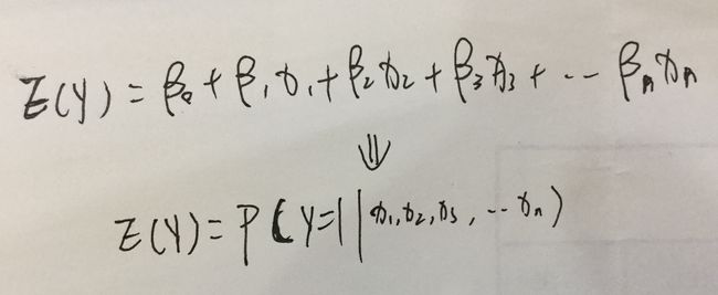
和线性回归一样,逻辑回归模型的自变量为各影响因素的线性组合,而因变量为某事件发生的概率。公式如下:
IMG_0743.jpg
然鹅。。。。
概率的值域范围是从0到1,所以需要对自变量线性函数组合进行函数对换,使改值域限制在0到1之间,这个函数如下:

IMG_0744.jpg
下面,我们利用R语言来实现逻辑回归
2.R语言的逻辑回归

2.jpg
2.1 案例一
#Customer:顾客序号
#Spending:消费金额(1000美元)
#Card:如果拥有VIP,则为1,否则为0
#Coupon:顾客使用了优惠券并购买了200美元或200美元以上的商品,则为1,否则为0

>data <- read.csv('./Simmons.csv')

>str(data)

## 'data.frame':    100 obs. of  4 variables:
##  $ Customer: int  1 2 3 4 5 6 7 8 9 10 ...
##  $ Spending: num  2.29 3.21 2.13 3.92 2.53 ...
##  $ Card    : int  1 1 1 0 1 0 0 0 1 0 ...
##  $ Coupon  : int  0 0 0 0 0 1 0 0 1 0 ...
查看数据类型,发现变量Card和Coupon是int类型,所以将其转化为因子型
>data$Card <- factor(data$Card,ordered = FALSE)
>data$Coupon <- factor(data$Coupon,ordered = FALSE)
>str(data)
## 'data.frame':    100 obs. of  4 variables:
##  $ Customer: int  1 2 3 4 5 6 7 8 9 10 ...
##  $ Spending: num  2.29 3.21 2.13 3.92 2.53 ...
##  $ Card    : Factor w/ 2 levels "0","1": 2 2 2 1 2 1 1 1 2 1 ...
##  $ Coupon  : Factor w/ 2 levels "0","1": 1 1 1 1 1 2 1 1 2 1 ...
2.1.1观察数据间的关系(其实觉得这步没啥必要,因为在模型中会去检验,就当做是学习吧)
#首先观察不同自变量与目标变量Coupon间是否存在显著的差异性
#由于Card是分类变量,所以使用列联表函数分析
>summary(table(data$Coupon,data$Card))$p.value #通过卡方检验,p值小于0.05,两者之间存在显著性差异,即Card很可能对vip的取值有影响
## [1] 0.01430588


#因为Spending是连续型数据,多以使用T检验来衡量二者之间的关系
>t.test(data$Spending[which(data$Coupon == 1)],data$Spending[which(data$Coupon==0)],paired = FALSE)$p.value #p值显示两者显著性差异
## [1] 0.007950012
2.1.2建立logic回归分析模型
>sol.glm <- glm(Coupon~Spending+Card,data=data,family = binomial(link='logit'))
>summary(sol.glm) #模型参数都通过了检验
##
## Call:
## glm(formula = Coupon ~ Spending + Card, family = binomial(link = "logit"),
##     data = data)
##
## Deviance Residuals:
##     Min       1Q   Median       3Q      Max
## -1.6839  -1.0140  -0.6503   1.1216   1.8794
##
## Coefficients:
##             Estimate Std. Error z value Pr(>|z|)
## (Intercept)  -2.1464     0.5772  -3.718 0.000201 ***
## Spending      0.3416     0.1287   2.655 0.007928 **
## Card1         1.0987     0.4447   2.471 0.013483 *
## ---
## Signif. codes:  0 '***' 0.001 '**' 0.01 '*' 0.05 '.' 0.1 ' ' 1
##
## (Dispersion parameter for binomial family taken to be 1)
##
##     Null deviance: 134.60  on 99  degrees of freedom
## Residual deviance: 120.97  on 97  degrees of freedom
## AIC: 126.97
##
## Number of Fisher Scoring iterations: 4
#这个仅仅只是为了学习step函数(对模型进行修正--步进)
>sol.glm<-step(sol.glm)
## Start:  AIC=126.97
## Coupon ~ Spending + Card
##
##            Df Deviance    AIC
##           120.97 126.97
## - Card      1   127.38 131.38
## - Spending  1   128.53 132.53

>summary(sol.glm)
##
## Call:
## glm(formula = Coupon ~ Spending + Card, family = binomial(link = "logit"),
##     data = data)
##
## Deviance Residuals:
##     Min       1Q   Median       3Q      Max
## -1.6839  -1.0140  -0.6503   1.1216   1.8794
##
## Coefficients:
##             Estimate Std. Error z value Pr(>|z|)
## (Intercept)  -2.1464     0.5772  -3.718 0.000201 ***
## Spending      0.3416     0.1287   2.655 0.007928 **
## Card1         1.0987     0.4447   2.471 0.013483 *
## ---
## Signif. codes:  0 '***' 0.001 '**' 0.01 '*' 0.05 '.' 0.1 ' ' 1
##
## (Dispersion parameter for binomial family taken to be 1)
##
##     Null deviance: 134.60  on 99  degrees of freedom
## Residual deviance: 120.97  on 97  degrees of freedom
## AIC: 126.97
##
## Number of Fisher Scoring iterations: 4
2.1.3逻辑回归模型常用输出项解读

IMG_0740_看图王.jpg
2.1.4模型预测和性能衡量
#预测
predict.coupon <- ifelse(sol.glm$fitted.values>=0.5,1,0)
predict.coupon<-as.factor(predict.coupon)
#对新数据进行预测
Spending <- sample(1:7,100,replace = TRUE)
Card <- as.factor(sample(c(0,1),100,replace = TRUE))
newdata <- data.frame(Spending=Spending,Card=Card)

new.predict.coupon <- predict(sol.glm,newdata = newdata) #因为预测结果是对数机会比,并不是概率
new.predict.coupon <- 1/(1+exp(-new.predict.coupon)) #将对数转换为概率

#前面两句可以用下面一句来代替
new.predict.coupon <- predict(sol.glm,newdata = newdata,type="response")


new.predict.coupon <- as.factor(ifelse(new.predict.coupon>=0.5,1,0))

#模型的衡量--预测准确率
length(which((predict.coupon==data$Coupon)==TRUE))/nrow(data)
## [1] 0.72
代码这么多,终于结束了。。。。。

2.jpg
但是就这么一个案例,难道就能将逻辑回归给掌握了?呵呵,要真是这样,岂不是人人都像吾一样有(S)才(B),那世界上就不会存在出轨了!
我ca,怎么一篇技术文扯到出轨了!这是我强行承上启下(小学语文老师教的真好,我居然还记得)

2.jpg
好吧,不扯淡了,下面这个案例来自《R语言实战》,思路承袭,但是也加了自己的一点东西
2.2 案例2
2.2.1查看数据
>data(Affairs,package='AER')
>summary(Affairs)
##     affairs          gender         age         yearsmarried    children
##  Min.   : 0.000   female:315   Min.   :17.50   Min.   : 0.125   no :171
##  1st Qu.: 0.000   male  :286   1st Qu.:27.00   1st Qu.: 4.000   yes:430
##  Median : 0.000                Median :32.00   Median : 7.000
##  Mean   : 1.456                Mean   :32.49   Mean   : 8.178
##  3rd Qu.: 0.000                3rd Qu.:37.00   3rd Qu.:15.000
##  Max.   :12.000                Max.   :57.00   Max.   :15.000
##  religiousness     education       occupation        rating
##  Min.   :1.000   Min.   : 9.00   Min.   :1.000   Min.   :1.000
##  1st Qu.:2.000   1st Qu.:14.00   1st Qu.:3.000   1st Qu.:3.000
##  Median :3.000   Median :16.00   Median :5.000   Median :4.000
##  Mean   :3.116   Mean   :16.17   Mean   :4.195   Mean   :3.932
##  3rd Qu.:4.000   3rd Qu.:18.00   3rd Qu.:6.000   3rd Qu.:5.000
##  Max.   :5.000   Max.   :20.00   Max.   :7.000   Max.   :5.000
>table(Affairs$affairs)
##
##   0   1   2   3   7  12
## 451  34  17  19  42  38
2.2.2转换数据类型
>Affairs$affairs[Affairs$affairs > 0] <- 1
>Affairs$affairs[Affairs$affairs == 0] <- 0
>Affairs$affairs <- factor(Affairs$affairs,levels = c(0,1),labels = c("No","Yes"))
>table(Affairs$affairs)
##
##  No Yes
## 451 150
>str(Affairs)
## 'data.frame':    601 obs. of  9 variables:
##  $ affairs      : Factor w/ 2 levels "No","Yes": 1 1 1 1 1 1 1 1 1 1 ...
##  $ gender       : Factor w/ 2 levels "female","male": 2 1 1 2 2 1 1 2 1 2 ...
##  $ age          : num  37 27 32 57 22 32 22 57 32 22 ...
##  $ yearsmarried : num  10 4 15 15 0.75 1.5 0.75 15 15 1.5 ...
##  $ children     : Factor w/ 2 levels "no","yes": 1 1 2 2 1 1 1 2 2 1 ...
##  $ religiousness: int  3 4 1 5 2 2 2 2 4 4 ...
##  $ education    : num  18 14 12 18 17 17 12 14 16 14 ...
##  $ occupation   : int  7 6 1 6 6 5 1 4 1 4 ...
##  $ rating       : int  4 4 4 5 3 5 3 4 2 5 ...
2.2.3将数据分为训练集和测试集
>library(caret)
## Loading required package: ggplot2
>splitIndex <- createDataPartition(Affairs$affairs,p=0.7,list=FALSE) #根据affairs的比例等比例抽样

>train_data <- Affairs[splitIndex,]
>test_data <- Affairs[-splitIndex,]
2.2.4构建模型
Aff.glm1 <- glm(affairs~.,data=train_data,family = binomial("logit"))
summary(Aff.glm1)
##
## Call:
## glm(formula = affairs ~ ., family = binomial("logit"), data = train_data)
##
## Deviance Residuals:
##     Min       1Q   Median       3Q      Max
## -1.4548  -0.7468  -0.5815  -0.2609   2.4321
##
## Coefficients:
##                Estimate Std. Error z value Pr(>|z|)
## (Intercept)    1.658817   1.063051   1.560 0.118658
## gendermale     0.402519   0.289301   1.391 0.164119
## age           -0.031756   0.021614  -1.469 0.141780
## yearsmarried   0.073137   0.037397   1.956 0.050505 .
## childrenyes    0.385327   0.346612   1.112 0.266270
## religiousness -0.378669   0.110115  -3.439 0.000584 ***
## education     -0.012741   0.060400  -0.211 0.832938
## occupation    -0.002265   0.088552  -0.026 0.979594
## rating        -0.396267   0.106665  -3.715 0.000203 ***
## ---
## Signif. codes:  0 '***' 0.001 '**' 0.01 '*' 0.05 '.' 0.1 ' ' 1
##
## (Dispersion parameter for binomial family taken to be 1)
##
##     Null deviance: 472.94  on 420  degrees of freedom
## Residual deviance: 431.62  on 412  degrees of freedom
## AIC: 449.62
##
## Number of Fisher Scoring iterations: 4
#查看之前的结果,有很多变量对方程的贡献不显著(原假设:参数为0)。去除这些变量重新拟合模型,检验新模型是否拟合的好
Aff.glm2 <- step(Aff.glm1)
## Start:  AIC=449.62
## affairs ~ gender + age + yearsmarried + children + religiousness +
##     education + occupation + rating
##
##                 Df Deviance    AIC
## - occupation     1   431.62 447.62
## - education      1   431.67 447.67
## - children       1   432.87 448.87
## - gender         1   433.57 449.57
##                431.62 449.62
## - age            1   433.86 449.86
## - yearsmarried   1   435.51 451.51
## - religiousness  1   443.89 459.89
## - rating         1   445.59 461.59
##
## Step:  AIC=447.62
## affairs ~ gender + age + yearsmarried + children + religiousness +
##     education + rating
##
##                 Df Deviance    AIC
## - education      1   431.69 445.69
## - children       1   432.91 446.91
##                431.62 447.62
## - gender         1   433.82 447.82
## - age            1   433.87 447.87
## - yearsmarried   1   435.52 449.52
## - religiousness  1   443.95 457.95
## - rating         1   445.60 459.60
##
## Step:  AIC=445.69
## affairs ~ gender + age + yearsmarried + children + religiousness +
##     rating
##
##                 Df Deviance    AIC
## - children       1   433.04 445.04
##                431.69 445.69
## - gender         1   433.98 445.98
## - age            1   434.06 446.06
## - yearsmarried   1   435.58 447.58
## - religiousness  1   443.96 455.96
## - rating         1   446.06 458.06
##
## Step:  AIC=445.04
## affairs ~ gender + age + yearsmarried + religiousness + rating
##
##                 Df Deviance    AIC
##                433.04 445.04
## - age            1   435.50 445.50
## - gender         1   435.69 445.69
## - yearsmarried   1   440.02 450.02
## - religiousness  1   445.33 455.33
## - rating         1   448.34 458.34
summary(Aff.glm2)
##
## Call:
## glm(formula = affairs ~ gender + age + yearsmarried + religiousness +
##     rating, family = binomial("logit"), data = train_data)
##
## Deviance Residuals:
##     Min       1Q   Median       3Q      Max
## -1.4577  -0.7538  -0.5873  -0.2862   2.3775
##
## Coefficients:
##               Estimate Std. Error z value Pr(>|z|)
## (Intercept)    1.66762    0.72035   2.315 0.020612 *
## gendermale     0.39749    0.24545   1.619 0.105352
## age           -0.03290    0.02137  -1.540 0.123653
## yearsmarried   0.08988    0.03448   2.607 0.009141 **
## religiousness -0.37500    0.10891  -3.443 0.000575 ***
## rating        -0.40991    0.10559  -3.882 0.000104 ***
## ---
## Signif. codes:  0 '***' 0.001 '**' 0.01 '*' 0.05 '.' 0.1 ' ' 1
##
## (Dispersion parameter for binomial family taken to be 1)
##
##     Null deviance: 472.94  on 420  degrees of freedom
## Residual deviance: 433.04  on 415  degrees of freedom
## AIC: 445.04
##
## Number of Fisher Scoring iterations: 4
#由step函数的结果来看,我们你可以选择一下变量进行建模
Aff.glm3 <-glm(formula = affairs ~ gender + age + yearsmarried + religiousness + rating, family = binomial("logit"), data = train_data)
summary(Aff.glm3)
##
## Call:
## glm(formula = affairs ~ gender + age + yearsmarried + religiousness +
##     rating, family = binomial("logit"), data = train_data)
##
## Deviance Residuals:
##     Min       1Q   Median       3Q      Max
## -1.4577  -0.7538  -0.5873  -0.2862   2.3775
##
## Coefficients:
##               Estimate Std. Error z value Pr(>|z|)
## (Intercept)    1.66762    0.72035   2.315 0.020612 *
## gendermale     0.39749    0.24545   1.619 0.105352
## age           -0.03290    0.02137  -1.540 0.123653
## yearsmarried   0.08988    0.03448   2.607 0.009141 **
## religiousness -0.37500    0.10891  -3.443 0.000575 ***
## rating        -0.40991    0.10559  -3.882 0.000104 ***
## ---
## Signif. codes:  0 '***' 0.001 '**' 0.01 '*' 0.05 '.' 0.1 ' ' 1
##
## (Dispersion parameter for binomial family taken to be 1)
##
##     Null deviance: 472.94  on 420  degrees of freedom
## Residual deviance: 433.04  on 415  degrees of freedom
## AIC: 445.04
##
## Number of Fisher Scoring iterations: 4
#Aff.glm3的有两个回归系数不显著(p>0.05).由于两模型嵌套(Aff.glm3是Aff.glm1的子集),对他们两个进行比较,对于广义线性模型,可用卡方检验
anova(Aff.glm3,Aff.glm1,test='Chisq')
## Analysis of Deviance Table
##
## Model 1: affairs ~ gender + age + yearsmarried + religiousness + rating
## Model 2: affairs ~ gender + age + yearsmarried + children + religiousness +
##     education + occupation + rating
##   Resid. Df Resid. Dev Df Deviance Pr(>Chi)
## 1       415     433.04
## 2       412     431.62  3   1.4156   0.7019
#看结果卡方值不显著(p=0.7019>0.05),表明去掉那几个变量的新模型和原先的模型的拟合程度一样好
2.2.5查看模型回归系数
Aff.glm3$coefficients
##   (Intercept)    gendermale           age  yearsmarried religiousness
##    1.66761680    0.39749043   -0.03290389    0.08988143   -0.37500013
##        rating
##   -0.40990588
#在Logistic回归中,相应变量是Y=1的对数机会比,因为对数解释性差,所以对结果指数化
exp(Aff.glm3$coefficients)
##   (Intercept)    gendermale           age  yearsmarried religiousness
##     5.2995229     1.4880856     0.9676315     1.0940446     0.6872892
##        rating
##     0.6637127
2.2.6检验过度离势
- 抽样于二项分布的数据的期望方差是σ 2 =nπ(1–π),n为观测数,π为属于Y=1组的概率。所谓 过度离势,即观测到的响应变量的方差大于期望的二项分布的方差。过度离势会导致奇异的标准 误检验和不精确的显著性检验
fit <- glm(affairs ~ age + yearsmarried + religiousness + rating, family = binomial(), data = train_data)
fit.od <- glm(affairs ~ age + yearsmarried + religiousness +rating, family = quasibinomial(), data = train_data)
pchisq(summary(fit.od)$dispersion*fit$df.residual,fit$df.residual,lower=F)
#结果不显著(p>0.05),不存在过度离势
## [1] 0.2841919
2.2.7利用测试集预测并查看准确率
aff_pre <- predict(Aff.glm3,newdata = test_data,type="response")

aff_pre <- factor(ifelse(aff_pre>=0.5,1,0),levels=c(0,1),labels=c("No","Yes"))

length(which(aff_pre==test_data$affairs)==TRUE)/nrow(test_data)
## [1] 0.7722222