聚类分析是在没有给出确定的划分类别的情况下,按照数据的相似度或者自身的距离进行样本分组的一种非监督方法。划分原则就是组内距离最小化而组间距离最大化。
K-Means算法:
基于距离的非层次聚类算法(划分方法),在目标函数最小化的基础上将数据划分成K类,数据点距离越近,相似度就越大,越容易被划为一类。K-Means算法的时间复杂度是O(tkn),其中t是循环次数;k是聚类个数;n是样本个数。由于t,k都要小于n,所以化简后为O(n).
算法实现:
1. 从样本数据中随机选择K个对象作为其实的中心点
2. 计算每个样本到所有中心点的距离,将样本分配到距离最近的聚类簇中
3. 所有样本分配完成后再次计算K个簇的中心
4. 如果簇的中心改变,则重新分配样本至距离最近的簇中直到最后聚类中心不再改变
聚类的结果对于初始中心点的选择具有随机性,所以最后的结果可能严重偏离全局最优解(对数据噪声和异常值很敏感)。因此,为了获得较好的结果,通常随机选择不同的初始聚类中心,多次运行K-Means算法。
对于连续数值:
样本相似性的度量中,一般采用欧氏距离;样本与簇之间的距离可以用样本到簇中心点的距离表示;同样,簇与簇之间的距离也是用簇中心的距离来代替。
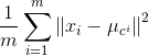
代价函数J(连续数值):
m个样本点距离所属聚类中心μc_i距离的平均平方和,优化的目标是使代价函数最小:
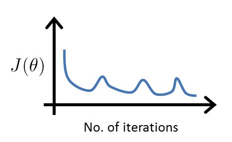
下图为代价函数在簇中心移动时的变化情况
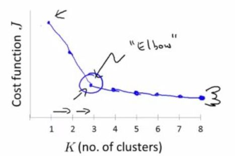
决定聚类数量:
通常需要人工判别,在无提前定义类别数的情况下,参考肘部原则Elbow method:
在预处理阶段需要对样本进行标准化(z-score normalization), 新数据符合标准正态分布,即均值为0,标准差为1.
聚类算法评价:(判断聚类结果的优劣)
簇内相似性越大,簇间差别越大,聚类的效果越好。
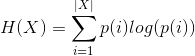
1. Purity评价:计算正确聚类数占总数的比例
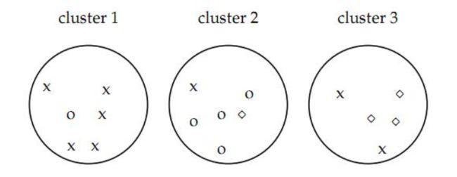
purity = (5+4+3)/17
2. Rand Index RI评价:用排列组合的原理进行评价的手段, RI取值范围为[0,1],RI越大表示聚类效果准确性越高 同时每个类内的纯度越高
TP是指被聚在一类的两个文档被正确分类了,TN是指不应该被聚在一类的两个文档被正确分开了,FP指不应该放在一类的文档被错误的放在了一类,FN指不应该分开的文档被错误的分开了。
按照上图例子:cluster1 = x, cluster2 = o, cluster3 = ◇ or x
cluster1 - 是x并且放在cluster1: C(2,5)
cluster2 - 是x并且放在cluster2: C(2,4)
cluster3 - 是x/◇并且放在cluster3: C(2,3)+C(2,2)
所以:TP = C(2,5) + C(2,4) + C(2,3) + C(2,2) = 20
C(2, 7) – Cluster 1 – test says ‘x’, so count those that are NOT x (and are correctly clustered in clusters 2 & 3),
C(2, 10) – Cluster 2, count those that are NOT ‘o’s and correctly clustered in clusters 1 & 3,
C(2, 4) – Cluster 3, count those that are NOT ‘x’ and NOT ‘d’(diamond shaped element)s that are correctly clustered in clusters 1& 2.
所以:TN = C(2,7) + C(2,10) + C(2,4) = 72
TP+TN+FP+FN = C(2, n_samples) = C(2,17) = 136
所以:RI = ( 20 + 72) / 136 = 0.68
*FP, FN可以不参与求解RI,但是可以通过如果转换得到:
The three clusters contain 6, 6, and 5 points, respectively, so the total number of ''positives'' or pairs of documents that are in the same cluster is
所以:TP+FP = C(2,6) + C(2,6) + C(2,5) = 15 + 15 + 10 = 40 其中C(n,m)是指在m中任选n个的组合数。
FP = 40 - 20 = 20
FN = C(2,17) - (TP+FP) - TN = 136 - 40 -72 = 24
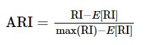
3. 调整兰德函数Adjusted Rand Index:the adjusted Rand index can yield negative values if the index is less than the expected index. Value is in [-1, 1].
The contingency table
Given a set S of n elements, and two groupings or partitions (e.g. clusterings) of these elements, namely X={x1,x2,...,xr} and Y={y1,y2,...,ys} , the overlap between X and Y can be summarized in a contingency table [nij] where each entry nij denotes the number of objects in common between Xi and Yi: nij = |Xi ∩ Yi|


4. F值评价:基于RI衍生
p = TP / (TP+FP), r = TP / (TP+FN)
The Rand index gives equal weight to false positives and false negatives. Separating similar documents is sometimes worse than putting pairs of dissimilar documents in the same cluster. We can use the F measure to penalize false negatives more strongly than false positives by selecting a valuea > 1, thus giving more weight to recall召回率.
5. 互信息mutual information评价:
是用来衡量两个数据分布的吻合程度。也是一类有用的信息度量,它是指两个事件集合之间的相关性。
设随机变量(X,Y)的联合分布为 p(x,y), 边际分布为 p(x),p(y), 互信息 I(X;Y) 是联合分布 p(x,y) 与 边际分布p(x),p(y)的相对熵,即:
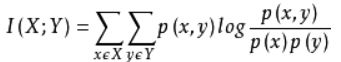
互信息越大,样本和聚类类别的关系就越大。
标准化后的互信息:
与ARI类似,调整互信息: