【Tensorflow】多分类问题的Precision、Recall和F1计算及Tensorflow实现

一、二分类问题的Precision、Recall、F1

网络上关于Precision、Recall和F1的介绍有很多，因此这里只作简单回顾。
在二分类问题中，根据真实类别和预测类别的组合可以分为四中情况，分别是TP(True Positive)、FP(False Positive)、TN(True Negative)、FN(False Negative)。如下图：

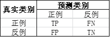
那么Precision表示所有被预测为Positive样本中，真正的Positive比例，即$Precision=\frac{TP}{TP+FP}$。

而Recall表示所有Positive样本中，被正确预测出来的比例，即$Recall=\frac{TP}{TP+FN}$。

F1则是Precision和Recall的调和平均数，即$F1=\frac{2PR}{P+R}$。

二、多分类问题的Precision、Recall和F1

显然，在多分类中没有了TP、FN、FP、TN的定义了。那么如何计算Precision、Recall和F1呢？下面介绍两种方式。

2.1 方法一：micro average

该方法的核心思想是将多个类别分组，真正关心的类别分为Positive组，其他分为Negative组。例如在命名实体识别任务中，将所有实体的类别分为Positive组，而其他标签’O’单独分为Negative组。下面以多分类的混淆矩阵(confuse matrix)为基础计算Precision、Recall和F1值。
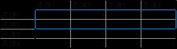
下图是多分类问题的混淆矩阵：

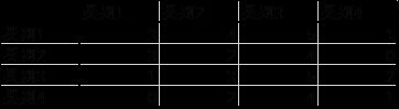
其中，假设类别1和类别2是Positive组，类别3和类别4是Negative组。
那么真正例(TP)可以定义为Positive组预测正确的样本数，那么下图红色框矩阵的对角线和(黄色单元格的和)即为真正例(TP)

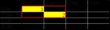
即TP=3+2=5

TP+FP表示所有被预测为Positive的样本数，显然下图红框中所有数的和就是TP+FP

即TP+FP=3+3+1+0+4+2+3+2=18

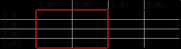
TP+FN表示所有真实为Positive的样本数，显然下图蓝色框中所有数的和就是TP+FN

即TP+FN=3+4+5+1+3+2+4+0=22

因此

$Precision=\frac{TP}{TP+FP}=\frac{5}{18}$

$Recall=\frac{TP}{TP+FN}=\frac{5}{22}$

$F1=\frac{2PR}{P+R}=\frac{1}{4}$

2.2 方法二：macro average

该方法的核心思想是，单独计算各个正例的Precison、Recall和F1，然后对所有正例的Precison、Recall和F1求平均值。
这里我们仍然将类别1和类别2作为Positive组，然后按上面的mincro分别计算类别1和类别2的Precison、Recall和F1。

2.2.1 计算类别1的Precision、Recall和F1

TP = 3

TP + FP = 3 + 3 + 1 + 0 = 7

TP + FN = 3 + 4 + 5 + 1 = 13

$Precisio{n}_1=\frac{TP}{TP+FP}=\frac{3}{7}$

$Recal{l}_1=\frac{TP}{TP+FN}=\frac{3}{13}$

$F{1}_1=\frac{2PR}{P+R}=\frac{3}{10}$

2.2.2 计算类别2的Precision、Recall和F1

TP = 2

TP + FP = 4 + 2 + 3 + 2 = 11

TP + FN = 3 + 2 + 4 + 0 = 9

$Precisio{n}_2=\frac{TP}{TP+FP}=\frac{2}{11}$

$Recal{l}_2=\frac{TP}{TP+FN}=\frac{2}{9}$

$F{1}_2=\frac{2PR}{P+R}=\frac{1}{5}$

2.2.3 计算平均值

$Precision=\frac{Precisio{n}_1+Precisio{n}_2}{2}=\frac{3/7+2/11}{2}=0.305$

$Recall=\frac{Recal{l}_1+Recal{l}_2}{2}=\frac{3/13+2/9}{2}=0.226$

$F1=\frac{F{1}_1+F{1}_2}{2}=\frac{3/10+1/5}{2}=0.25$

三、Tensorflow实现

import tensorflow as tf
import numpy as np
from tensorflow.python.ops.metrics_impl import _streaming_confusion_matrix

1、计算混淆矩阵(confuse matrix)

labels = tf.convert_to_tensor(np.array([0,0,1,1,2,2]))
predictions = tf.convert_to_tensor(np.array([0,1,2,0,0,1]))
num_classes = 3  # 3个类别0,1,2
# cm是上一个batch的混淆矩阵，op是更新完当前batch的
cm,op = _streaming_confusion_matrix(labels,predictions,num_classes)

with tf.Session() as sess:
    sess.run(tf.local_variables_initializer()) # 初始化所有的local variables
    print(sess.run(cm))
    print(sess.run(op))
cm = op # 令cm是更新后的混淆矩阵

[[0. 0. 0.]
 [0. 0. 0.]
 [0. 0. 0.]]
[[1. 1. 0.]
 [1. 0. 1.]
 [1. 1. 0.]]

2、计算micro average的precision、recall和f1

def safe_div(numerator, denominator):
    """安全除，分母为0时返回0"""
    numerator, denominator = tf.cast(numerator,dtype=tf.float64), tf.cast(denominator,dtype=tf.float64)
    zeros = tf.zeros_like(numerator, dtype=numerator.dtype) # 创建全0Tensor
    denominator_is_zero = tf.equal(denominator, zeros) # 判断denominator是否为零
    return tf.where(denominator_is_zero, zeros, numerator / denominator) # 如果分母为0，则返回零

def pr_re_f1(cm, pos_indices):
    num_classes = cm.shape[0]
    neg_indices = [i for i in range(num_classes) if i not in pos_indices]
    cm_mask = np.ones([num_classes, num_classes])
    cm_mask[neg_indices, neg_indices] = 0 # 将负样本预测正确的位置清零零
    diag_sum = tf.reduce_sum(tf.diag_part(cm * cm_mask)) # 正样本预测正确的数量

    cm_mask = np.ones([num_classes, num_classes])
    cm_mask[:, neg_indices] = 0 # 将负样本对应的列清零
    tot_pred = tf.reduce_sum(cm * cm_mask) # 所有被预测为正的样本数量

    cm_mask = np.ones([num_classes, num_classes])
    cm_mask[neg_indices, :] = 0 # 将负样本对应的行清零
    tot_gold = tf.reduce_sum(cm * cm_mask) # 所有正样本的数量

    pr = safe_div(diag_sum, tot_pred)
    re = safe_div(diag_sum, tot_gold)
    f1 = safe_div(2. * pr * re, pr + re)
    
    return pr, re, f1

pr,re,f1 = pr_re_f1(cm,[0,1])
with tf.Session() as sess:
    sess.run(tf.local_variables_initializer())
    print(sess.run(pr))
    print(sess.run(re))
    print(sess.run(f1))

0.2
0.25
0.22222222222222224

3、计算macro average的precision、recall和f1

precisions, recalls, f1s, n_golds = [], [], [], []
pos_indices = [0,1] # 正例
# 计算每个正例的precison,recall和f1
for idx in pos_indices:
    pr, re, f1 = pr_re_f1(cm, [idx])
    precisions.append(pr)
    recalls.append(re)
    f1s.append(f1)
    cm_mask = np.zeros([num_classes, num_classes])
    cm_mask[idx, :] = 1
    n_golds.append(tf.to_float(tf.reduce_sum(cm * cm_mask)))
pr = tf.reduce_mean(precisions)
re = tf.reduce_mean(recalls)
f1 = tf.reduce_mean(f1s)

with tf.Session() as sess:
    sess.run(tf.local_variables_initializer())
    print(sess.run(pr))
    print(sess.run(re))
    print(sess.run(f1))

0.16666666666666666
0.25
0.2