Tensorflow2.0之门控循环单元(GRU)原理与实现
文章目录
- GRU 介绍
- 门控循环单元
- 重置门和更新门
- 候选隐藏状态
- 隐藏状态
- 输出结果
- 代码实现
- 1、导入需要的库
- 2、加载周杰伦歌词数据集
- 3、定义采样函数
- 3.1 随机采样
- 3.2 相邻采样
- 4、one-hot向量
- 5、初始化模型参数
- 6、定义模型
- 6.1 初始化隐藏状态
- 6.2 在一个时间步里计算隐藏状态和输出
- 7、定义预测函数
- 8、裁剪梯度
- 9、定义模型训练函数
- 9.1 困惑度
- 9.2 初始化优化器
- 9.3 定义梯度下降函数
- 9.4 定义训练函数
- 9.5 训练
- Tensorflow2.0 实现GRU
- 参考资料
GRU 介绍
循环神经网络中如何通过时间反向传播?中介绍了循环神经网络中的梯度计算方法。我们发现,当时间步数较大或者时间步较小时,循环神经网络的梯度较容易出现衰减或爆炸。虽然裁剪梯度可以应对梯度爆炸,但无法解决梯度衰减的问题。通常由于这个原因,循环神经网络在实际中较难捕捉时间序列中时间步距离较大的依赖关系。
门控循环单元
门控循环神经网络(gated recurrent neural network)的提出,正是为了更好地捕捉时间序列中时间步距离较大的依赖关系。它通过可以学习的门来控制信息的流动。其中,门控循环单元(gated recurrent unit,GRU)是一种常用的门控循环神经网络。
重置门和更新门
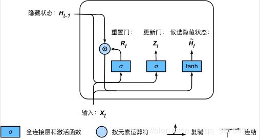
如下图所示,门控循环单元中的重置门和更新门的输入均为当前时间步输入 X t \boldsymbol{X}_t Xt 与上一时间步隐藏状态 H t − 1 \boldsymbol{H}_{t-1} Ht−1,输出由激活函数为 sigmoid 函数的全连接层计算得到。
 具体来说,假设样本数为 n n n、输入个数为 d d d(即每个样本包含的元素数,一般为词典大小)、隐藏单元个数为 h h h,给定时间步 t t t 的小批量输入 X t ∈ R n × d \boldsymbol{X}_t \in \mathbb{R}^{n \times d} Xt∈Rn×d 和上一时间步隐藏状态 H t − 1 ∈ R n × h \boldsymbol{H}_{t-1} \in \mathbb{R}^{n \times h} Ht−1∈Rn×h。重置门 R t ∈ R n × h \boldsymbol{R}_t \in \mathbb{R}^{n \times h} Rt∈Rn×h 和更新门 Z t ∈ R n × h \boldsymbol{Z}_t \in \mathbb{R}^{n \times h} Zt∈Rn×h 的计算如下:
R t = σ ( X t W x r + H t − 1 W h r + b r ) \boldsymbol{R}_t = \sigma(\boldsymbol{X}_t \boldsymbol{W}_{xr} + \boldsymbol{H}_{t-1} \boldsymbol{W}_{hr} + \boldsymbol{b}_r) Rt=σ(XtWxr+Ht−1Whr+br)
Z t = σ ( X t W x z + H t − 1 W h z + b z ) \boldsymbol{Z}_t = \sigma(\boldsymbol{X}_t \boldsymbol{W}_{xz} + \boldsymbol{H}_{t-1} \boldsymbol{W}_{hz} + \boldsymbol{b}_z) Zt=σ(XtWxz+Ht−1Whz+bz)
其中 W x r , W x z ∈ R d × h \boldsymbol{W}_{xr}, \boldsymbol{W}_{xz} \in \mathbb{R}^{d \times h} Wxr,Wxz∈Rd×h 和 W h r , W h z ∈ R h × h \boldsymbol{W}_{hr}, \boldsymbol{W}_{hz} \in \mathbb{R}^{h \times h} Whr,Whz∈Rh×h 是权重参数, b r , b z ∈ R 1 × h \boldsymbol{b}_r, \boldsymbol{b}_z \in \mathbb{R}^{1 \times h} br,bz∈R1×h 是偏差参数。sigmoid 函数可以将元素的值变换到0和1之间。因此,重置门 R t \boldsymbol{R}_t Rt 和更新门 Z t \boldsymbol{Z}_t Zt 中每个元素的值域都是 [ 0 , 1 ] [0, 1] [0,1]。
候选隐藏状态
接下来,门控循环单元将计算候选隐藏状态来辅助稍后的隐藏状态计算。如下图所示,我们将当前时间步重置门的输出与上一时间步隐藏状态做按元素乘法(符号为 ⊙ \odot ⊙)。如果重置门中元素值接近0,那么意味着重置对应隐藏状态元素为0,即丢弃上一时间步的隐藏状态。如果元素值接近1,那么表示保留上一时间步的隐藏状态。然后,将按元素乘法的结果与当前时间步的输入连结,再通过含激活函数 tanh 的全连接层计算出候选隐藏状态,其所有元素的值域为 [ − 1 , 1 ] [-1, 1] [−1,1]。
具体来说,时间步 t t t 的候选隐藏状态 H ~ t ∈ R n × h \tilde{\boldsymbol{H}}_t \in \mathbb{R}^{n \times h} H~t∈Rn×h 的计算为:
H ~ t = tanh ( X t W x h + ( R t ⊙ H t − 1 ) W h h + b h ) \tilde{\boldsymbol{H}}_t = \text{tanh}(\boldsymbol{X}_t \boldsymbol{W}_{xh} + \left(\boldsymbol{R}_t \odot \boldsymbol{H}_{t-1}\right) \boldsymbol{W}_{hh} + \boldsymbol{b}_h) H~t=tanh(XtWxh+(Rt⊙Ht−1)Whh+bh)
其中 W x h ∈ R d × h \boldsymbol{W}_{xh} \in \mathbb{R}^{d \times h} Wxh∈Rd×h 和 W h h ∈ R h × h \boldsymbol{W}_{hh} \in \mathbb{R}^{h \times h} Whh∈Rh×h 是权重参数, b h ∈ R 1 × h \boldsymbol{b}_h \in \mathbb{R}^{1 \times h} bh∈R1×h 是偏差参数。从上面这个公式可以看出,重置门控制了上一时间步的隐藏状态如何流入当前时间步的候选隐藏状态。而上一时间步的隐藏状态可能包含了时间序列截至上一时间步的全部历史信息。因此,重置门可以用来丢弃与预测无关的历史信息从而有助于捕捉时间序列里短期的依赖关系
隐藏状态
最后,时间步 t t t 的隐藏状态 H t ∈ R n × h \boldsymbol{H}_t \in \mathbb{R}^{n \times h} Ht∈Rn×h 的计算使用当前时间步的更新门 Z t \boldsymbol{Z}_t Zt 来对上一时间步的隐藏状态 H t − 1 \boldsymbol{H}_{t-1} Ht−1 和当前时间步的候选隐藏状态 H ~ t \tilde{\boldsymbol{H}}_t H~t 做组合:
H t = Z t ⊙ H t − 1 + ( 1 − Z t ) ⊙ H ~ t \boldsymbol{H}_t = \boldsymbol{Z}_t \odot \boldsymbol{H}_{t-1} + (1 - \boldsymbol{Z}_t) \odot \tilde{\boldsymbol{H}}_t Ht=Zt⊙Ht−1+(1−Zt)⊙H~t
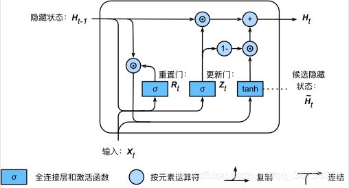 值得注意的是,更新门可以控制隐藏状态应该如何被包含当前时间步信息的候选隐藏状态所更新,如上图所示。假设更新门在时间步 t ′ t' t′ 到 t t t( t ′ < t t' < t t′<t)之间一直近似于1。那么,在时间步 t ′ t' t′ 到 t t t 之间的输入信息几乎没有流入时间步 t t t 的隐藏状态 H t \boldsymbol{H}_t Ht。实际上,这可以看作是较早时刻的隐藏状态 H t ′ − 1 \boldsymbol{H}_{t'-1} Ht′−1 一直通过时间保存并传递至当前时间步 t t t。这个设计可以应对循环神经网络中的梯度衰减问题,并更好地捕捉时间序列中时间步距离较大的依赖关系(即长期的依赖关系)。
输出结果
将上面得到的隐藏状态 H t H_t Ht 输入神经网络,得到结果 Y t ∈ R n × q \boldsymbol{Y}_t \in \mathbb{R}^{n \times q} Yt∈Rn×q:
Y t = H t W h q + b q \boldsymbol{Y}_t = \boldsymbol{H}_t \boldsymbol{W}_{hq} + \boldsymbol{b}_q Yt=HtWhq+bq
总结来说:
- 重置门有助于捕捉时间序列里短期的依赖关系;
- 更新门有助于捕捉时间序列里长期的依赖关系。
代码实现
在这个部分,我们将从零开始实现一个基于门控循环单元的语言模型,并在周杰伦专辑歌词数据集上训练一个模型来进行歌词创作。
1、导入需要的库
import tensorflow as tf
from tensorflow import keras
import numpy as np
import zipfile
import math
2、加载周杰伦歌词数据集
def load_data_jay_lyrics():
    with zipfile.ZipFile('./jaychou_lyrics.txt.zip') as zin:
        with zin.open('jaychou_lyrics.txt') as f:
            corpus_chars = f.read().decode('utf-8')
    corpus_chars = corpus_chars.replace('\n', ' ').replace('\r', ' ')
    corpus_chars = corpus_chars[0:10000]
    idx_to_char = list(set(corpus_chars))
    char_to_idx = dict([(char, i) for i, char in enumerate(idx_to_char)])
    vocab_size = len(char_to_idx)
    corpus_indices = [char_to_idx[char] for char in corpus_chars]
    return corpus_indices, char_to_idx, idx_to_char, vocab_size

(corpus_indices, char_to_idx, idx_to_char, vocab_size) = load_data_jay_lyrics()
对这一部分以及下一部分的采样有疑惑的小伙伴请移步至:Tensorflow2.0之语言模型数据集(周杰伦专辑歌词)预处理。
3、定义采样函数
3.1 随机采样
def data_iter_random(corpus_indices, batch_size, num_steps):
    num_examples = (len(corpus_indices)-1) // num_steps
    epoch_size = num_examples // batch_size
    example_indices = list(range(num_examples))
    random.shuffle(example_indices)

    # 返回从pos开始的长为num_steps的序列
    def _data(pos):
        return corpus_indices[pos: pos + num_steps]

    for i in range(epoch_size):
        # 每次读取batch_size个随机样本
        i = i * batch_size
        batch_indices = example_indices[i: i + batch_size]
        X = [_data(j * num_steps) for j in batch_indices]
        Y = [_data(j * num_steps + 1) for j in batch_indices]
        yield np.array(X), np.array(Y)
3.2 相邻采样
def data_iter_consecutive(corpus_indices, batch_size, num_steps, ctx=None):
    corpus_indices = np.array(corpus_indices)
    data_len = len(corpus_indices)
    batch_len = data_len // batch_size
    indices = corpus_indices[0: batch_size*batch_len].reshape((
        batch_size, batch_len))
    epoch_size = (batch_len - 1) // num_steps
    for i in range(epoch_size):
        i = i * num_steps
        X = indices[:, i: i + num_steps]
        Y = indices[:, i + 1: i + num_steps + 1]
        yield X, Y

data_iter = data_iter_consecutive(corpus_indices, batch_size=32, num_steps=35)
4、one-hot向量
为了将词表示成向量输入到神经网络,一个简单的办法是使用one-hot向量,即独热编码。假设词典中不同字符的数量为 N N N(即词典大小vocab_size),每个字符已经和一个从0到 N − 1 N-1 N−1的连续整数值索引一一对应,包含这些一一对应的字符及其索引值的字典是第二部分得到的 char_to_idx。如果一个字符的索引是整数 i i i, 那么我们创建一个全0的长为 N N N的向量,并将位置为 i i i的元素设成1。该向量就是对原字符的one-hot向量。
我们每次采样的小批量的形状是(批量大小, 时间步数)。下面的函数将这样的小批量变换成数个可以输入进网络的形状为 (批量大小, 词典大小) 的矩阵,矩阵个数等于时间步数。也就是说,时间步 t t t的输入为 X t ∈ R n × d \boldsymbol{X}_t \in \mathbb{R}^{n \times d} Xt∈Rn×d,其中 n n n为批量大小, d d d为输入个数,即one-hot向量长度(词典大小)。
def to_onehot(X, size):
    # X shape: (batch, steps), output shape: (batch, vocab_size)
    return [tf.one_hot(x, size,dtype=tf.float32) for x in X.T]
举例来说:
X = np.arange(10).reshape((2, 5))
inputs = to_onehot(X, vocab_size)
那么 X 为:
[[0 1 2 3 4]
 [5 6 7 8 9]]
是一个包含两个 batch,且时间步长为5的数据。也就是说,第一个时间点的输入为0和5,第二个时间点的输入为1和6,以此类推。
经过 one-hot 变换后得到的 inputs 为:
[<tf.Tensor: id=9, shape=(2, 1027), dtype=float32, numpy=
array([[1., 0., 0., ..., 0., 0., 0.],
       [0., 0., 0., ..., 0., 0., 0.]], dtype=float32)>, <tf.Tensor: id=14, shape=(2, 1027), dtype=float32, numpy=
array([[0., 1., 0., ..., 0., 0., 0.],
       [0., 0., 0., ..., 0., 0., 0.]], dtype=float32)>, <tf.Tensor: id=19, shape=(2, 1027), dtype=float32, numpy=
array([[0., 0., 1., ..., 0., 0., 0.],
       [0., 0., 0., ..., 0., 0., 0.]], dtype=float32)>, <tf.Tensor: id=24, shape=(2, 1027), dtype=float32, numpy=
array([[0., 0., 0., ..., 0., 0., 0.],
       [0., 0., 0., ..., 0., 0., 0.]], dtype=float32)>, <tf.Tensor: id=29, shape=(2, 1027), dtype=float32, numpy=
array([[0., 0., 0., ..., 0., 0., 0.],
       [0., 0., 0., ..., 0., 0., 0.]], dtype=float32)>]
包含了5个时间点的数据,第一个时间点的数据是0和5的独热编码,以此类推。
5、初始化模型参数
根据上文中对循环神经网络的介绍,我们可以得到所有参数(权重和阈值)的 shape:
- W x h ∈ R d × h \boldsymbol{W}_{xh} \in \mathbb{R}^{d \times h} Wxh∈Rd×h
- W h h ∈ R h × h \boldsymbol{W}_{hh} \in \mathbb{R}^{h \times h} Whh∈Rh×h
- b h ∈ R 1 × h \boldsymbol{b}_h \in \mathbb{R}^{1 \times h} bh∈R1×h
- W h q ∈ R h × q \boldsymbol{W}_{hq} \in \mathbb{R}^{h \times q} Whq∈Rh×q
- b q ∈ R 1 × q \boldsymbol{b}_q \in \mathbb{R}^{1 \times q} bq∈R1×q
其中, d d d 指的是每个(经过独热编码后的)输入样本的维度,即词典的大小; h h h 指的是隐藏层中的神经元个数; q q q 指的是输出向量的维度,由于输出向量中包含着下一个时间点选择各个字符的概率,所以 q q q 也等于词典大小。
num_epochs, num_steps = 2500, 35
num_inputs, num_hiddens, num_outputs = vocab_size, 256, vocab_size
def get_params():
    def _one(shape):
        return tf.Variable(tf.random.normal(shape=shape,
                                             stddev=0.01,
                                             mean=0,
                                             dtype=tf.float32))
    def _three():
        return (_one(shape=(num_inputs, num_hiddens)),
                 _one(shape=(num_hiddens, num_hiddens)),
                 tf.Variable(tf.zeros(shape=(num_hiddens, ), dtype=tf.float32)))

    W_xr, W_hr, b_r = _three()
    W_xz, W_hz, b_z = _three()
    W_xh, W_hh, b_h = _three()
    W_hq = _one(shape=(num_hiddens, num_outputs))
    b_q = tf.Variable(tf.zeros(shape=(num_outputs, ), dtype=tf.float32))
    params = [W_xr, W_hr, b_r, W_xz, W_hz, b_z, W_xh, W_hh, b_h, W_hq, b_q]

    return params
6、定义模型
在定义模型之前,我们要先对一个时间点上的输入数据及隐藏状态的 shape 进行归纳:
- X t ∈ R n × d \boldsymbol{X}_t \in \mathbb{R}^{n \times d} Xt∈Rn×d
- H t ∈ R n × h \boldsymbol{H}_t \in \mathbb{R}^{n \times h} Ht∈Rn×h
其中, n n n指的是每批样本的个数; d d d 指的是每个(经过独热编码后的)输入样本的维度,即词典的大小; h h h 指的是隐藏层中的神经元个数。
6.1 初始化隐藏状态
我们根据循环神经网络的计算表达式实现该模型。首先定义 init_rnn_state 函数来返回初始化的隐藏状态。它返回由一个形状为 (批量大小, 隐藏单元个数) 的所有值都为0的数组。
# 返回初始化的隐藏状态
def init_gru_state(batch_size):
    return (tf.zeros(shape=(batch_size, num_hiddens)), )
6.2 在一个时间步里计算隐藏状态和输出
这里的激活函数使用了 tanh 函数,因为当元素在实数域上均匀分布时,tanh 函数值的均值为0。
def gru(inputs, state, params):
    W_xz, W_hz, b_z, W_xr, W_hr, b_r, W_xh, W_hh, b_h, W_hq, b_q = params
    H, = state
    outputs = []
    for X in inputs:
        X=tf.reshape(X,[-1,W_xh.shape[0]])
        Z = tf.sigmoid(tf.matmul(X, W_xz) + tf.matmul(H, W_hz) + b_z)
        R = tf.sigmoid(tf.matmul(X, W_xr) + tf.matmul(H, W_hr) + b_r)
        H_tilda = tf.tanh(tf.matmul(X, W_xh) + tf.matmul(R * H, W_hh) + b_h)
        H = Z * H + (1 - Z) * H_tilda
        Y = tf.matmul(H, W_hq) + b_q
        outputs.append(Y)
    return outputs, (H,)
在上面的函数中,inputs 和 outputs 皆为 num_steps 个形状为 (batch_size, vocab_size) 的矩阵,每次循环只对其中一个矩阵进行计算。
在进行训练时,inputs 的形状为 (batch_size, vocab_size),但是在进行预测时,inputs 的形状为 (1, vocab_size),所以要先将 X 的形状转换为 (-1, vocab_size),否则 X 的形状就是 (vocab_size,) 从而不能进行下面的操作了。
如:
A = np.array([[1, 2, 3, 4, 5, 6]])
print(A.shape)
for a in A:
    print(a.shape)
(1, 6)
(6,)
7、定义预测函数
以下函数基于前缀 prefix(含有数个字符的字符串)来预测接下来的 num_chars 个字符。
def predict_rnn(prefix, num_chars, params):
    state = init_gru_state(batch_size=1)
    output = [char_to_idx[prefix[0]]]
    for t in range(num_chars + len(prefix) - 1):
        # 将上一时间步的输出作为当前时间步的输入
        X = tf.convert_to_tensor(to_onehot(np.array([output[-1]]), vocab_size),dtype=tf.float32)
#         print(X.shape)
#         X = tf.reshape(X,[1,-1])
        # 计算输出和更新隐藏状态
        (Y, state) = gru(X, state, params)
#         print(Y)
        # 下一个时间步的输入是prefix里的字符或者当前的最佳预测字符
        if t < len(prefix) - 1:
            output.append(char_to_idx[prefix[t + 1]])
        else:
            output.append(int(np.array(tf.argmax(Y[0],axis=1))))
    return ''.join([idx_to_char[i] for i in output])
我们可以先试验一下:
params = get_params()
print(predict_rnn('分开', 10, params))
得到:
分开盯欠袋王中写鸥油村丛
因为模型参数为随机值,所以预测结果也是随机的。
8、裁剪梯度
循环神经网络中较容易出现梯度衰减或梯度爆炸。为了应对梯度爆炸,我们可以裁剪梯度(clip gradient)。假设我们把所有模型参数梯度的元素拼接成一个向量 g \boldsymbol{g} g,并设裁剪的阈值是 θ \theta θ。裁剪后的梯度
min ( θ ∣ g ∣ , 1 ) g \min\left(\frac{\theta}{|\boldsymbol{g}|}, 1\right)\boldsymbol{g} min(∣g∣θ,1)g
的 L 2 L_2 L2范数不超过 θ \theta θ。
def grad_clipping(grads,theta):
    norm = np.array([0])
    for i in range(len(grads)):
        norm+=tf.math.reduce_sum(grads[i] ** 2)
    norm = np.sqrt(norm).item()
    new_gradient=[]
    if norm > theta:
        for grad in grads:
            new_gradient.append(grad * theta / norm)
    else:
        for grad in grads:
            new_gradient.append(grad)
    return new_gradient
9、定义模型训练函数
跟之前的模型训练函数相比,这里的模型训练函数有以下几点不同:
- 使用困惑度评价模型。
- 在迭代模型参数前裁剪梯度。
- 对时序数据采用不同采样方法将导致隐藏状态初始化的不同。
9.1 困惑度
我们通常使用困惑度(perplexity)来评价语言模型的好坏。困惑度是对交叉熵损失函数做指数运算后得到的值。特别地,
- 最佳情况下,模型总是把标签类别的概率预测为1,此时困惑度为1;
- 最坏情况下,模型总是把标签类别的概率预测为0,此时困惑度为正无穷;
- 基线情况下,模型总是预测所有类别的概率都相同,此时困惑度为类别个数。
显然,任何一个有效模型的困惑度必须小于类别个数。在本例中,困惑度必须小于词典大小vocab_size。
9.2 初始化优化器
optimizer = tf.keras.optimizers.SGD(learning_rate=1e2)
9.3 定义梯度下降函数
def train_step(params, X, Y, state, clipping_theta):
    with tf.GradientTape(persistent=True) as tape:
        tape.watch(params)
        inputs = to_onehot(X, vocab_size)
        # outputs有num_steps个形状为(batch_size, vocab_size)的矩阵
        (outputs, state) = gru(inputs, state, params)
        # 拼接之后形状为(num_steps * batch_size, vocab_size)
        outputs = tf.concat(outputs, 0)
        # Y的形状是(batch_size, num_steps),转置后再变成长度为
        # batch * num_steps 的向量,这样跟输出的行一一对应
        y = Y.T.reshape((-1,))
        y = tf.convert_to_tensor(y, dtype=tf.float32)
        # 使用交叉熵损失计算平均分类误差
        l = tf.reduce_mean(tf.losses.sparse_categorical_crossentropy(y, outputs))

    grads = tape.gradient(l, params)
    grads = grad_clipping(grads, clipping_theta)  # 裁剪梯度
    optimizer.apply_gradients(zip(grads, params))
    return l, y
9.4 定义训练函数
- is_random_iter:是否随机采样;
- pred_period:间隔多少次展示一次结果;
- pred_len:要求预测的字符长度。
def train_and_predict_rnn(is_random_iter, batch_size, clipping_theta, pred_period, pred_len, prefixes):
    if is_random_iter:
        data_iter_fn = data_iter_random
    else:
        data_iter_fn = data_iter_consecutive
    params = get_params()

    for epoch in range(num_epochs):
        if not is_random_iter:  # 如使用相邻采样,在epoch开始时初始化隐藏状态
            state = init_gru_state(batch_size)
        l_sum, n = 0.0, 0
        data_iter = data_iter_fn(corpus_indices, batch_size, num_steps)
        for X, Y in data_iter:
            if is_random_iter:  # 如使用随机采样,在每个小批量更新前初始化隐藏状态
                state = init_gru_state(batch_size)
            l, y = train_step(params, X, Y, state, clipping_theta)
            l_sum += np.array(l).item() * len(y)
            n += len(y)

        if (epoch + 1) % pred_period == 0:
            print('epoch %d, perplexity %f' % (epoch + 1, math.exp(l_sum / n)))
            for prefix in prefixes:
                print(prefix)
                print(' -', predict_rnn(prefix, pred_len, params))
9.5 训练
pred_period, pred_len, prefixes = 50, 50, ['分开', '不分开']
clipping_theta = 0.01
batch_size = 32
train_and_predict_rnn(False, batch_size, clipping_theta, pred_period, pred_len, prefixes)
Tensorflow2.0 实现GRU
在Tensorflow2.0之用循环神经网络生成周杰伦歌词中,我们已经用 Tensorflow2.0 中提供的高级 API 实现了循环神经网络,在这里,我们只需要修改实例化 RNN 的部分即可。
也就是将:
cell = keras.layers.SimpleRNNCell(num_hiddens,
                                  kernel_initializer='glorot_uniform')
rnn_layer = keras.layers.RNN(cell,time_major=True,
                            return_sequences=True,return_state=True)
修改为:
rnn_layer = keras.layers.GRU(num_hiddens,time_major=True,
                            return_sequences=True,return_state=True)
参考资料
门控循环单元(GRU)