机器学习笔记(14)——sklearn降维方法举例(RandomProjection,TSVD,t-SNE)

sklearn降维方法举例

以datasets.digits数据为例导入相关包

import numpy as np
import pandas as pd
import matplotlib.pyplot as plt
import time
from sklearn.datasets import load_digits

大样本数据的可视化是一个相对比较麻烦的事情，
一般情况下我们都要用到降维的方法先处理特征。我们找一个例子来看看，可以怎么做，比如我们数据集取经典的『手写数字集』
Each datapoint is a 8x8 image of a digit.
Classes->10
Samples per class->180
Samples total->1797
Dimensionality->64
Features integers->0-16

导入数据,0,1,2,3,4,5,6这7个数字的手写图像

digits = load_digits(n_class=7)#integer
X = digits.data
y = digits.target
n_samples,n_features = X.shape

输出图像

from matplotlib import offsetbox
def plot_embedding(X, title=None):
    x_min, x_max = np.min(X, 0), np.max(X, 0)
    X = (X - x_min) / (x_max - x_min)#正则化
    print X
    plt.figure(figsize=(10, 10))
    ax = plt.subplot(111)
    for i in range(X.shape[0]):
        plt.text(X[i, 0], X[i, 1], str(digits.target[i]),
                 color=plt.cm.Set1(y[i] / 10.),
                 fontdict={'weight': 'bold', 'size': 12})
    #打印彩色字体
    if hasattr(offsetbox, 'AnnotationBbox'):
        # only print thumbnails with matplotlib > 1.0
        shown_images = np.array([[1., 1.]])  # just something big
        for i in range(digits.data.shape[0]):
            dist = np.sum((X[i] - shown_images) ** 2, 1)
            if np.min(dist) < 4e-3:
                # don't show points that are too close
                continue
            shown_images = np.r_[shown_images, [X[i]]]
            imagebox = offsetbox.AnnotationBbox(
                offsetbox.OffsetImage(digits.images[i], cmap=plt.cm.gray_r),
                X[i])
            ax.add_artist(imagebox)#输出图上输出图片
    plt.xticks([]), plt.yticks([])
    if title is not None:
        plt.title(title)

1.随机投射(Random-Projection)

首先我们来看一个问题， 如果你手头有一组数据$X\in R^n$， 它的维数太高， 从而不得不进行降维至$R^k$， 你会怎么办？
相信不少人反射性地求它的$x’x$，然后转化为延最大方差展开的问题。 当然这个方法需要求解固有值和固有向量。对于测试用的小数据一切似乎都很好， 但如果我给你的是50G大小csv格式的Twitter发言呢？如果需要对全部单词降维， 恐怕半个月吧。 因此我们需要个更加快速的方法。
那么现在再来想， 既然要快， 那我们就用个最简单的方法： 随机在高维空间里选几个单位向量$e_i$， 但注意， 这里我们仅仅要求是单位向量， 并没有要求它们之间必须正交$<e_i,e_j>=0$， 因此你可以随便选。 最后， 我们把高维数据投影到选择的这一组基上。也就完成了降维。
随便选的轴如何能保证降维效果？ 但它是有数学依据的， 叫做Johnson-Lindenstrauss Lemma。这个定理保证了任何降维方法的精度上下限。
#####Johnson-Lindenstrauss Lemma
假设我们有数据$x\in R^n$， 而我们通过一种方法$f(x)$将其降维成$y\in R^k$， 那么， 将为前后任意两点$a,b$之间的距离有不等式保证：
$(1-ϵ)\Vert a-b{\Vert }^2\le \Vert f(a)-f(b){\Vert }^2\le (1+ϵ)\Vert a-b{\Vert }^2$
对于随机映射来说， 只要注意到下面几点就行了：

• 1.不定式中的精度仅仅受制于维数、数据大小等因素， 与将为方法无关。
• 2.在维数差不是很大时， 总可以保证一个相对较高的精度， 不论用什么方法。
• 3.到这里一切就很明显了， 既然精度有上界， 那我们也就不必担心轴的选取，那么最简单的方法自然就是随机挑选了， 这也就产生的Random Projection这一方法。

Random Projection

简单来说,Random Projection流程就是
选择影射矩阵$R\in {\mathcal{R}}^{K\times N}$。
用随机数填充影射矩阵。 可以选择uniform或者gaussian。
归一化每一个新的轴（影射矩阵中的每一行）。
对数据降维$y=R\mathcal{X}$。
上个小节里面的JL-lemma保证的降维的效果不会太差。
从直观上来看看。
首先假设我们有数据$\mathcal{X}=\{x|f^i(\theta )+\sigma \}$， 其中$\theta$是一组参数， $\sigma$则是高斯噪声。 回想PCA方法， 我们很自然的认为所有的特征都是正交的， 我们既没有考虑它是不是有多个中心， 也没有考虑是不是有特殊结构， 然而对于实际数据， 很多时候并不是这样。 比如我们把取$f(\theta )=S^i({\theta }_i)N(A,{\sigma }^i)\in R^3$， 其中$S^i\in SO(3)$， 这样我们得到的数据可能会像$\times$或者$\ast$一样， 显然用PCA并不能得到好的结果。
在这种情况下， 考虑在非常高维度的空间， 可以想象random projection这种撞大运的方法总会选到一些超平面能够接近数据的特征， 同时也能够想象如果目标维数过低， 那么命中的概率就会大大降低。

实现：

from sklearn import random_projection
rp = random_projection.SparseRandomProjection(n_components=2, random_state=42)
#随机映射算法
start_time = time.time()
X_projected = rp.fit_transform(X)#随机投射
plot_embedding(X_projected, "Random Projection of the digits (time: %.3fs)" % (time.time() - start_time))
plt.show()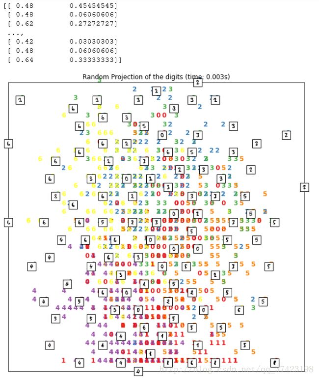

时间很短但效果一般

官方描述：

def sparse_random_matrix(n_components, n_features, density='auto',
                         random_state=None):
    """Generalized Achlioptas random sparse matrix for random projection

    Setting density to 1 / 3 will yield the original matrix by Dimitris
    Achlioptas while setting a lower value will yield the generalization
    by Ping Li et al.

    If we note :math:`s = 1 / density`, the components of the random matrix are
    drawn from:

      - -sqrt(s) / sqrt(n_components)   with probability 1 / 2s
      -  0                              with probability 1 - 1 / s
      - +sqrt(s) / sqrt(n_components)   with probability 1 / 2s

    Read more in the :ref:`User Guide `.

    Parameters
    ----------
    n_components : int,
        Dimensionality of the target projection space.

    n_features : int,
        Dimensionality of the original source space.

    density : float in range ]0, 1] or 'auto', optional (default='auto')
        Ratio of non-zero component in the random projection matrix.

        If density = 'auto', the value is set to the minimum density
        as recommended by Ping Li et al.: 1 / sqrt(n_features).

        Use density = 1 / 3.0 if you want to reproduce the results from
        Achlioptas, 2001.

    random_state : integer, RandomState instance or None (default=None)
        Control the pseudo random number generator used to generate the
        matrix at fit time.

    Returns
    -------
    components: numpy array or CSR matrix with shape [n_components, n_features]
        The generated Gaussian random matrix.
    """
    _check_input_size(n_components, n_features)
    density = _check_density(density, n_features)
    rng = check_random_state(random_state)

    if density == 1:
        # skip index generation if totally dense
        components = rng.binomial(1, 0.5, (n_components, n_features)) * 2 - 1
        return 1 / np.sqrt(n_components) * components

    else:
        # Generate location of non zero elements
        indices = []
        offset = 0
        indptr = [offset]
        for i in xrange(n_components):
            # find the indices of the non-zero components for row i
            n_nonzero_i = rng.binomial(n_features, density)
            indices_i = sample_without_replacement(n_features, n_nonzero_i,
                                                   random_state=rng)
            indices.append(indices_i)
            offset += n_nonzero_i
            indptr.append(offset)

        indices = np.concatenate(indices)

        # Among non zero components the probability of the sign is 50%/50%
        data = rng.binomial(1, 0.5, size=np.size(indices)) * 2 - 1

        # build the CSR structure by concatenating the rows
        components = sp.csr_matrix((data, indices, indptr),
                                   shape=(n_components, n_features))

        return np.sqrt(1 / density) / np.sqrt(n_components) * components

2.TSVD(截断奇异值分解, TruncatedSVD,PCA的一种实现)

截断奇异值分解（Truncated singular value decomposition，TSVD）是一种矩阵因式分解（factorization）技术，将矩阵 M 分解成 U ， Σ 和 V 。它与PCA很像，只是SVD分解是在数据矩阵上进行，而PCA是在数据的协方差矩阵上进行。通常，SVD用于发现矩阵的主成份。对于病态矩阵，目前主要的处理办法有预调节矩阵方法、区域分解法、正则化方法等，截断奇异值分解技术TSVD就是一种正则化方法，它牺牲部分精度换去解的稳定性，使得结果具有更高的泛化能力。
对于原始数据矩阵A(N*M) ，N代表样本个数，M代表维度，对其进行SVD分解：

$$A=U\Sigma V^T,\Sigma =diag({\delta }_1,{\delta }_2,\dots ,{\delta }_n)=\left[\begin{array}{cccccc}{\delta }_1& 0& 0& .& .& 0\\ 0& {\delta }_2& 0& .& .& 0\\ 0& 0& {\delta }_3& .& .& 0\\ .& .& .& .& .& .\\ .& .& .& .& .& .\\ 0& 0& 0& .& .& {\delta }_n\end{array}\right]$$

上式中的$\delta$就是数据的奇异值，且${\delta }_1$>${\delta }_2$>${\delta }_3$…，通常如果A非常病态，delta的后面就越趋向于0，$\frac{{\delta }_1}{{\delta }_n}$就是数据的病态程度，越大说明病态程度越高，无用的特征越多，通常会截取前p个最大的奇异值，相应的U截取前p列，V截取前p列，这样A依然是N*M的矩阵，用这样的计算出来的A代替原始的A，就会比原始的A更稳定。
TSVD与一般SVD不同的是它可以产生一个指定维度的分解矩阵。例如，有一个 n×n 矩阵，通过SVD分解后仍然是一个 n×n 矩阵，而TSVD可以生成指定维度的矩阵。这样就可以实现降维了。

演示一下TSVD工作原理

In[1]:
import numpy as np
from scipy.linalg import svd
D = np.array([[1, 2], [1, 3], [1, 4]])
D

Out[1]:
array([[1, 2],
       [1, 3],
       [1, 4]])

In[2]:
U, S, V = svd(D, full_matrices=False)
#我们可以根据SVD的定义，用 UU ， SS 和 VV 还原矩阵 DD 
U.shape, S.shape, V.shape

Out[2]:
((3, 2), (2, 1), (2, 2))

In[3]:
np.dot(U.dot(np.diag(S)), V)#还原

Out[3]:
array([[ 1.,  2.],
       [ 1.,  3.],
       [ 1.,  4.]])

TruncatedSVD返回的矩阵是 U 和 S 的点积。如果我们想模拟TSVD，我们就去掉最新奇异值和对于 U 的列向量。例如，我们想要一个主成份，可以这样：

In[4]:
new_S = S[0]
new_U = U[:, 0]
new_U.dot(new_S)

Out[4]:
array([-2.20719466, -3.16170819, -4.11622173])

TruncatedSVD有个“陷阱”。随着随机数生成器状态的变化，TruncatedSVD连续地拟合会改变输出的符合。为了避免这个问题，建议只用TruncatedSVD拟合一次，然后用其他变换。这正是管线命令的另一个用处。

实现：

from sklearn import decomposition
X_pca = decomposition.TruncatedSVD(n_components=2).fit_transform(X)
start_time = time.time()
plot_embedding(X_pca,"Principal Components projection of the digits (time: %.3fs)" % (time.time() - start_time))
plt.show()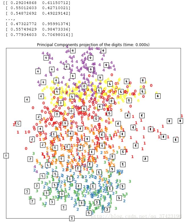

效果稍微好一些

3.t-SNE(t-分布邻域嵌入算法)

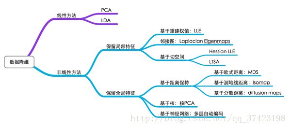
流形学习方法(Manifold Learning)，简称流形学习,可以将流形学习方法分为线性的和非线性的两种，线性的流形学习方法如我们熟知的主成份分析（PCA），非线性的流形学习方法如等距映射（Isomap）、拉普拉斯特征映射（Laplacian eigenmaps，LE）、局部线性嵌入(Locally-linear embedding，LLE)。

t-SNE详细介绍：http://lvdmaaten.github.io/tsne/

from sklearn import manifold
#降维
tsne = manifold.TSNE(n_components=2, init='pca', random_state=0)
start_time = time.time()
X_tsne = tsne.fit_transform(X)
#绘图
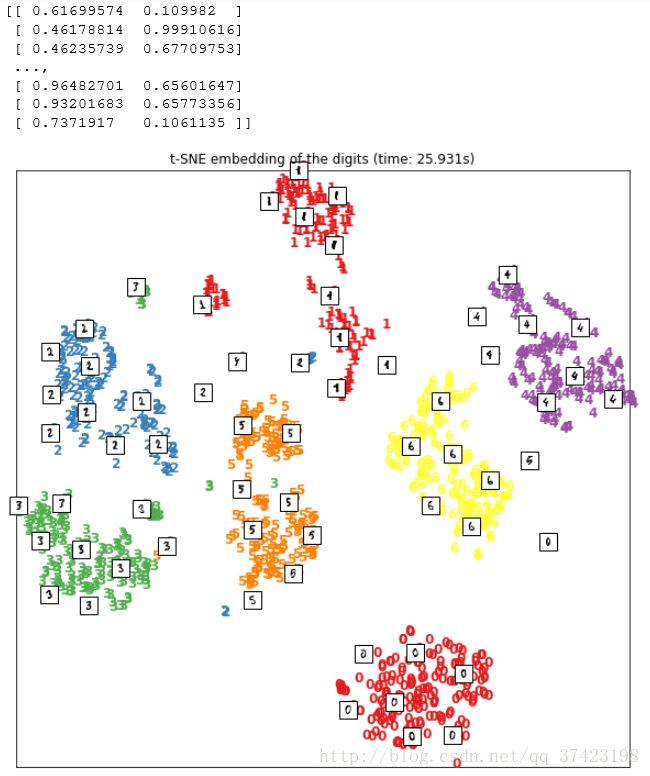
plot_embedding(X_tsne,
               "t-SNE embedding of the digits (time: %.3fs)" % (time.time() - start_time))
plt.show()
#这个非线性变换降维过后，仅仅2维的特征，就可以将原始数据的不同类别，在平面上很好地划分开。
#不过t-SNE也有它的缺点，一般说来，相对于线性变换的降维，它需要更多的计算时间。