TensorFlow2.0——模型构建

模型构建：

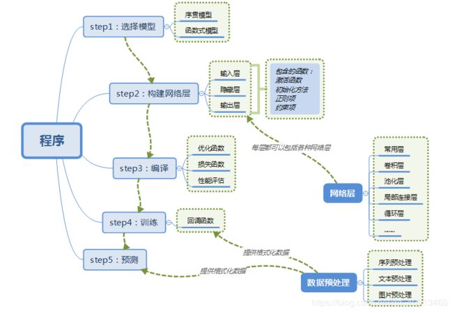
Keras有两种类型的模型，序贯模型（Sequential）和函数式模型（Model），函数式模型应用更为广泛，序贯模型是函数式模型的一种特殊情况。

a）序贯模型（Sequential):单输入单输出，一条路通到底，层与层之间只有相邻关系，没有跨层连接。这种模型编译速度快，操作也比较简单

b）函数式模型（Model）：多输入多输出，层与层之间任意连接。这种模型编译速度慢。

引用：https://blog.csdn.net/zjw642337320/article/details/81204560

代码示例：

引用必要的函数库：

import matplotlib as mpl
import matplotlib.pyplot as plt 
%matplotlib inline    
#为了能在notebook中显示图像
import numpy as np
import sklearn   #注意
import pandas as pd 
import os 
import sys 
import time 
import tensorflow as tf 

from tensorflow import keras 

1.选择模型并构建网络

#使用序贯模型Sequential   tf.keras.models.sequential()
'''第一种写法
model = keras.models.Sequential()#注意要大写，选择模型
#构建网络
model.add(keras.layers.Flatten(input_shape = [28,28])) #序贯模型的第一层需要输入数据的shape
model.add(keras.layers.Dense(300, activation = "relu"))#Dense 全连接层
model.add(keras.layers.Dense(100, activation = "relu"))
model.add(keras.layers.Dense(10, activation = "softmax")) 
'''

#第二种写法
model = keras.models.Sequential([
    keras.layers.Flatten(input_shape = [28, 28]),  #注意逗号
    keras.layers.Dense(300, activation="relu"),  
    keras.layers.Dense(100, activation="relu"),
    keras.layers.Dense(10, activation="softmax")
])

#softmax将向量变成概率分布   x = [xl, x2，x3].
# y = [e^x1/sum, e^x2/sum, e^x3/sum]    sum = e^x1 + e^x2 + e^x3

2.编译

#编译compile
model.compile(loss = "sparse_categorical_crossentropy",   
             optimizer = "adam", #优化函数，不直接使用梯度下降
             metrics = ["accuracy"]) 

loss 为损失函数；
sparse_categorical_crossentropy或者categorical_crossentropy，这两者都是多分类交差熵，区别在于：
sparse_categorical_crossentropy：tagets 是数字编码；
categorical_crossentropy：targets 是 one-hot 编码；

optimizer：优化函数，例如 AdamOptimizer、RMSPropOptimizer 或 GradientDescentOptimizer

metrics:性能评估，用于监控训练，它们是 tf.keras.metrics 模块中的字符串名称或可调用对象

查看模型信息：

model.layers  #查看一下网络的层次

运行结果：

[,
,
,
]

model.summary() # num = [none,784] * w + b -> [none,300]    W.shape[300,784] , b = [300]

Model: “sequential_1”

---

Layer (type)    Output Shape       Param #
===============================================================
flatten_1 (Flatten)   (None, 784)      0

---

dense_2 (Dense)    (None, 300)    235500

---

dense_3 (Dense)    (None, 100)    30100

---

dense_4 (Dense)    (None, 10)     1010
===============================================================
Total params: 266,610
Trainable params: 266,610
Non-trainable params: 0

---

3.训练模型

#训练模型
history = model.fit(x_train, y_train, epochs=10, validation_data=(x_valid, y_valid)) 
#会返回一个结果保存在history中

‘’’
model.fit的一些参数,参考官方API
batch_size：对总的样本数进行分组，每组包含的样本数量
epochs ：训练次数
shuffle：是否把数据随机打乱之后再进行训练
validation_split：拿出百分之多少用来做交叉验证
verbose：屏显模式 0：不输出 1：输出进度 2：输出每次的训练结果

查看history的类型

type(history)

tensorflow.python.keras.callbacks.History

history.history

{‘loss’: [2.456370598454909,
0.6194203653292223,
0.5326741259748285,
0.4874053767854517,
0.4296531865163283,
0.4044668952768499,
0.39407426077669316,
0.372555995017832,
0.36333005535169083,
0.35417791644118046],
‘accuracy’: [0.72492725,
0.7869091,
0.8126,
0.8274182,
0.8468909,
0.8547091,
0.8584727,
0.86585456,
0.8695273,
0.87316364],
‘val_loss’: [0.6873663679599762,
0.5281977466583252,
0.47626469302177427,
0.43247376172542573,
0.4234978169679642,
0.4271171735525131,
0.3985502668261528,
0.4447905594587326,
0.42555881497859954,
0.38597796664237977],
‘val_accuracy’: [0.783,
0.8132,
0.8464,
0.851,
0.863,
0.851,
0.8708,
0.8616,
0.859,
0.8706]}

绘制图形查看

def plot_learning_curves(history):
    pd.DataFrame(history.history).plot(figsize=(8,5))
    plt.grid(True)
    plt.show
    
plot_learning_curves(history)