自然语言处理：序列标注（BiLSTM-CRF）

Reference:

1. Bidirectional LSTM-CRF Models for Sequence Tagging
2. Neural Architectures for Named Entity Recognition
3. Character-based BiLSTM-CRF Incorporating POS and Dictionaries for Chinese Opinion Target Extraction
4. CRF Layer on the Top of BiLSTM
5. Bi-LSTM + CRF with character embeddings for NER and POS

Tagging Scheme

IOBES: Inside, Outside, Beginning, End, Single

Bidirectional LSTM Networks

By utilize bidirectional LSTM, we can efficiently make use of past features (via forward states) and future features (via backward states) for a specific time frame.

We train the bidirectional LSTM networks using BPTT, and specially treat at the beginning and the end of the data points. Such as reset the hidden states to 0 at the begging of each sentence.

At time $t$ for NER task:

• the input layer represents features could be one-hot-encoding for word feature, dense vector features, or sparse features.
• the output layer represents a probability distribution (distributed by softmax) over labels. It has the same dimensionality as size of labels. Using the label with the max probability as output of timestep $t$.

Why use the CRF Networks?

Despite use the ${\mathbf{h}}_t$ as features to make independent tagging decisions for each output $y_t$ is success in POS tagging, the independent classification decisions are limiting when there are strong dependencies across output labels.

As the NER task, since the “grammar” that characterizes interpretable sequences of tags imposes several hard constraints (e.g. I-PER cannot follow B-LOC) that would be impossible to model with independence assumptions.

The first way is to predict a distribution of tags of each time step and then use beam-like decoding to find optimal tag sequences, such as Maximum entropy classifier (Ratnaparkhi, 1996) and Maximum entropy Markov models (McCallum etal., 2000).

The second way is to focus on sentence level instead of individual positions, thus leading to Conditional Random Fields (CRF) models that the inputs and outputs are directly connected, as opposed to LSTM networks where memory cells/recurrent components are employed.

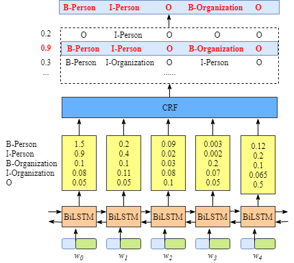
如下最右侧图，若不考虑不同位置词标注之间的关系，会出现错误的标注。

对于序列标注任务，输入词序列为观测序列，带标注的序列为隐藏状态序列。基于状态独立假设的序列标注模型，无法处理不同状态间的硬性约束，MRMM、CRF擅长解决此类问题。

MEMM假设当前状态仅与上一状态有关（马尔可夫性假设），CRF没有马尔可夫性假设，预测每个状态时考虑全局状态信息。

HMM（马尔可夫性假设、观测独立性假设） -> MEMM（马尔可夫性假设）-> CRF

CRF Networks

BiLSTM-CRF networks

Given $\mathbf{x}=(x_1,x_2,\cdots ,x_n)$ and $\mathbf{y}=(y_1,y_2,\cdots ,y_n)$ to represent an input sequence and a sequence of predicted tags respectively, where $n$ is the length of the input sentence.

Emission score

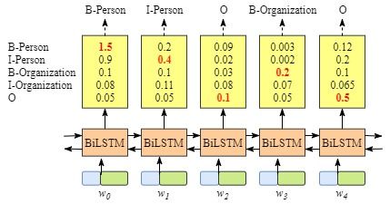
We consider $\mathbf{P}\in {\mathbb{R}}^{n\times k}$ to be the matrix of scores output by the BiLSTM network, where $k$ is the number of distinct tags, the element $P[i,j]$ corresponds to the score of the $j$-th tag of the $i$-th word in a sentence.

In BiLSTM-CRF networks, emission scores come from the BiLSTM layer. For instance, according the above figure, the score of $w_0$ labeled as B-Person is 1.5.

对于长度为$n$的句子，发射矩阵$P$包含$n$个$k$维的隐藏状态.

Transition score

CRF introduces a transition matrix $\mathbf{A}\in {\mathbb{R}}^{(k+2)\times (k+2)}$, that is position independent, which measure the score from $i$-th tag to $j$-th tag by the element $A[i,j]$.

In order to make the transition score matrix more robust, we will add the START and the END tags of a sentence to the set of possible tags. $\mathbf{A}$ is therefore a square matrix of size $k+2$.

Here is an example of the transition matrix score including the extra added START and END labels.

Transition Matrix	START	B-Person	I-Person	B-Organization	I-Organization	O	END
START	0	0.8	0.007	0.7	0.0008	0.9	0.08
B-Person	0	0.6	0.9	0.2	0.0006	0.6	0.009
I-Person	-1	0.5	0.53	0.55	0.0003	0.85	0.008
B-Organization	0.9	0.5	0.0003	0.25	0.8	0.77	0.006
I-Organization	-0.9	0.45	0.007	0.7	0.65	0.76	0.2
O	0	0.65	0.0007	0.7	0.0008	0.9	0.08
END	0	0	0	0	0	0	0

As shown in the table above, we can find that the transition matrix has learned some useful constraints.

• The label of first word in a sentence should start with “B-” or “O”, not “I-”.
• etc.

Where or how to get the transition matrix?

Transition matrix is a parameter of CRF layer. It’s initialization with random value, that will be more and more reasonable gradually with increasing training iterations.

Decoding

For a sentence has 5 words: $x_1,x_2,x_3,x_4,x_5$, the real tags $\mathbf{y}$ is:

"START B-Person I-Person O B-Organization O END"

Here, we add two more extra words which denote the start and the end of sentence: $x_0,x_6$.

A linear-chain CRF defines a global score $s(\mathbf{x},\mathbf{y})$ consists of 2 parts, such that:
$$s(\mathbf{x},\mathbf{y})=s_e(\mathbf{x},\mathbf{y})+s_t(\mathbf{y})=\sum _{i=1}^{n}P[x_i,y_i]+\sum _{i=0}^{n}A[y_i,y_{i+1}]$$

Emission Score
$$s_e(\mathbf{x},\mathbf{y})=P[x_0,\text{START}]+P[x_1,\text{B-Person}]+\cdots +P[x_6,\text{END}]$$

where $P_0$ and $P_6$ just set them zeros, $P_1\cdots P_5$ are from the previous BiLSTM.

Transition Score
$$s_t(\mathbf{y})=A[\text{START},\text{B-Person}]+A[\text{B-Person},\text{I-Person}]+\cdots +A[\text{O},\text{END}]$$

these score are actually the parameters of CRF layer.

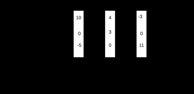
Illustration of the scoring of a sentence with linear-chain CRF:

The path PER-O-LOC has a score of: 1 + 10 + 4 + 3 + 2 + 11 + 0 = 31

The path PER-PER-LOC has a score of: 1 + 10 + 2 + 4 - 2 + 11 + 0 = 26

Now that we understand the scoring function of the CRF, we need to do 2 things:

• Find the sequence of tags with the best score.
• Compute a probability distribution over all the sequence of tags (total score).

The simplest way to measure the total score is that: enumerating all the possible paths and sum their scores. However, it is very inefficient, with $n^k$ complexity. The recurrent nature of our formula makes it the perfect candidates to apply dynamic programming.

维特比算法求解最优路径

Let’s suppose that $c_t(y_t,\mathbf{x})$ is the solution for time steps $t,\cdots ,n$ for sequences that start with $y_t$:

$$\begin{array}{rl}{c}_t(y_t,\mathbf{x})& ={\arg \max }_{y_t,\cdots ,y_n}s(y_t,\cdots y_n,\mathbf{x})\\ & ={\arg \max }_{y_t,\cdots ,y_n}P[x_t,y_t]+A[y_t,y_{t+1}]+s(y_{t+1},\cdots ,y_n,\mathbf{x})\\ & =\arg {\max }_{y_{t+1}}P[x_t,y_t]+A[y_t,y_{t+1}]+c_{t+1}(y_{t+1},\mathbf{x})\end{array}$$
The best score and path are:
$$s(\mathbf{x},{\mathbf{y}}^{\ast })=c_0(y_0=\text{START},\mathbf{x})，{\mathbf{y}}^{\ast }=\arg \underset{\tilde{\mathbf{y}}\in Y}{\max }s(\mathbf{x},\tilde{\mathbf{y}})$$
As we perform $n$ step, final cost is $O(n{k}^2)$, much less than $O(k^n)$.

类似于CRF解码（已知模型、观测求最可能的状态序列）的维特比算法

动态规划求解归一化因子

模型的优化目标是最大化目标标注序列的概率，一般使用softmax将分数转化为概率，softmax分母项需求解所有可能标注序列的分数和$Z$，也称为归一化因子，下面介绍基于前向递推动态规划的优化求解算法。
$$p(\mathbf{y}|\mathbf{x})=\frac{1}{Z}\exp (s(\mathbf{x},\mathbf{y})),Z=\sum _{\tilde{\mathbf{y}}}\exp (s(\mathbf{x},\tilde{\mathbf{y}}))$$
假定已知时刻$t$以$y_t$为标注结尾的所有可能标注序列的总分数为$Z_t(y_t)$，即
$$\begin{array}{rl}{Z}_t(y_t)& =\sum _{y_1,\cdots ,y_{t-1}}\exp (s(y_1,\cdots ,y_t,\mathbf{x}))\\ & =\sum _{y_{t-1}}\exp (P[x_t,y_t]+A[y_{t-1},y_t])\sum _{y_1,\cdots ,y_{t-2}}\exp (s(y_1,\cdots ,y_{t-1}))\\ & =\sum _{y_{t-1}}\exp (P[x_t,y_t]+A[y_{t-1},y_t])\cdot Z_{t-1}(y_{t-1})\end{array}$$
对于总时间步为$n$的序列，所有可能标注序列的总分数为
$$Z=\sum _{y_n}{Z}_n(y_n)$$

动态规划求解对数归一化因子

归一化因子需对n条路径求指数和，很容易造成浮点数溢出，实际优化函数也是极大化目标序列的对数似然
$$\log p(\mathbf{y}|\mathbf{x})=s(\mathbf{x},\mathbf{y})-\log \sum _{\tilde{\mathbf{y}}}\exp (s(\mathbf{x},\tilde{\mathbf{y}}))$$
令$Z_t(y_t)$表示时刻$t$以$y_t$结尾的所有可能序列分数的logsumexp，则前向递归公式为（这边文章用实例说明的很好）
$$\begin{array}{rl}{Z}_t(y_t)& =\log \sum _{y_1\cdots y_{t-1}}{e}^{s(\mathbf{x},y_1\cdots y_t)}\\ & =\log \sum _{y_{t-1}}{e}^{P[x_t,y_t]+A[y_{t-1},y_t]}\sum _{y_1\cdots y_{t-2}}{e}^{s(\mathbf{x},y_1\cdots y_{t-1})}\\ & =\log \sum _{y_{t-1}}{e}^{P[x_t,y_t]+A[y_{t-1},y_t]}{e}^{Z_{t-1}(y_{t-1})}\\ & =\log \sum _{y_{t-1}}{e}^{P[x_t,y_t]+A[y_{t-1},y_t]+Z_{t-1}(y_{t-1})}\end{array}$$
任意时刻$t$对所有的$Z_t(y_t)$再进行一次logsumexp，得到该时刻总分数的对数归一化因子
$$Z_t=\log \sum _{y_t}{e}^{Z_t(y_t)}=\log \sum _{y_1\cdots y_t}{e}^{s(\mathbf{x},y_1\cdots y_t)}$$

神奇的公式

很多文献、博客中介绍归一化因子对数形式的递推公式时，引入公式
$$\log \sum e^{\log (\sum e^x)+y}=\log \sum \sum e^{x+y}$$
这个公式很难理解，为什么可以根据这个公式就能得到对应归一化因子的递推公式？

不难发现，本文中的$Z_t(y_t)$的递推公式中的第4、2行分别对应这个公式左右两个方程，其中
$$y=P[x_t,y_t]+A[y_{t-1},y_t],x=s(x,y_1\cdots y_{t-1}),Z_{t-1}(y_{t-1})=\log \sum e^x$$

logsumexp防止溢出性

很容易证明，以下等式成立
$$\log \sum _x{e}^x=a+\log \sum _x{e}^{x-a}$$
令$a=\max x$ 就不会造成数据上溢出，softmax函数多采用这种处理。

Loss function

CRF loss function is consist of the real path score and the total score of all the possible paths. The real path should having the highest score among those of all possible paths.

The loss function of CRF model as below (minimize loss function):
$$L(\theta )=-\log p(\mathbf{y}|\mathbf{x})=-s(\mathbf{x},\mathbf{y})+{\text{logadd}}_{\tilde{\mathbf{y}}\in Y}s(\mathbf{x},\tilde{\mathbf{y}})$$

where the score $s(\mathbf{x},\mathbf{y})$ of real path should be the one with largest percentage in all the scores, $Y$ represents all possible tag sequences, even those that do not verify the IOB format for a sentence $\mathbf{x}$.

During the training process, the parameter values of our BiLSTM-CRF model will be updated again and again to keep increasing the percentage of the score of the real path.

Bi-LSTM-CRF Networks

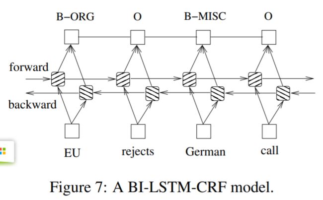
Combine a Bi-LSTM network and a CRF network to form a Bi-LSTM-CRF model. This network can efficiently use past input features via a Bi-LSTM layer and sentence level tag information via a CRF layer.

We construct our neural network by using hidden state of Bi-LSTM layer as input sequence of CRF layer. We can use the concatenation hidden states (forward + backward), denoted as ${\mathbf{h}}_t$ of $x_t$ to predict the tag of corrected $x_t$ directly, since it contains the context information.

We feed those hidden states $\mathbf{h}=({\mathbf{h}}_1,{\mathbf{h}}_2,\cdots ,{\mathbf{h}}_n)$ into CRF layer:
$$\mathbf{P}={\mathbf{W}}_s\mathbf{h}+{\mathbf{b}}_s$$

where ${\mathbf{W}}_s$ and ${\mathbf{b}}_s$ are the parameters.