《机器学习实战》笔记——第三章:决策树实战
1 说明
该书主要以原理简介+项目实战为主,本人学习的主要目的是为了结合李航老师的《统计学习方法》以及周志华老师的西瓜书的理论进行学习,从而走上机器学习的“不归路”。因此,该笔记主要详细进行代码解析,从而透析在进行一项机器学习任务时候的思路,同时也积累自己的coding能力。
正文由如下几部分组成:
1、实例代码(详细注释)
2、知识要点(函数说明)
3、调试及结果展示
2 正文
(1)计算给定数据集的信息熵
1、给定数据集为:
def createDataSet():
    dataSet = [[1, 1, 'yes'],
               [1, 1, 'yes'],
               [1, 0, 'no'],
               [0, 1, 'no'],
               [0, 1, 'no']]
    labels = ['no surfacing','flippers']
    #change to discrete values
    return dataSet, labels
该函数将书中表3-1海洋生物数据存在了一个python列表中,方便后续的处理。
接下来我们定义一个calcShannonEnt函数来计算香农信息熵:
def calcShannonEnt(dataSet):
    numEntries = len(dataSet)#获取数据集样本个数
    labelCounts = {}#初始化一个字典用来保存每个标签出现的次数
    for featVec in dataSet:
        currentLabel = featVec[-1]#逐个获取标签信息
        # 如果标签没有放入统计次数字典的话,就添加进去
        if currentLabel not in labelCounts.keys(): labelCounts[currentLabel] = 0
        labelCounts[currentLabel] += 1
    shannonEnt = 0.0#初始化香农熵
    for key in labelCounts:
        prob = float(labelCounts[key])/numEntries#选择该标签的概率
        shannonEnt -= prob * log(prob,2)#公式计算
    return shannonEnt
2、在python命令提示符下输入下列命令:
******
PyDev console: starting.
Python 3.6.7 |Anaconda, Inc.| (default, Oct 28 2018, 19:44:12) [MSC v.1915 64 bit (AMD64)] on win32
>>>import trees
>>>myDat, labels = trees.createDataSet()
>>>myDat
[[1, 1, 'yes'], [1, 1, 'yes'], [1, 0, 'no'], [0, 1, 'no'], [0, 1, 'no']]
>>>trees.calcShannonEnt(myDat)
0.9709505944546686
>>>myDat[0][-1] = 'maybe'
>>>myDat
[[1, 1, 'maybe'], [1, 1, 'yes'], [1, 0, 'no'], [0, 1, 'no'], [0, 1, 'no']]
>>>trees.calcShannonEnt(myDat)
1.3709505944546687
我们可以看到,在数据集中添加更多的分类,信息熵明显变大了。
知识要点:
①信息熵:是度量样本集合纯度最常用的一种指标,信息的期望值。
《机器学习》(周志华 著):假定当前样本集合D中第k类样本所占的比例为 p k ( k = 1 , 2 , … , ∣ γ ∣ ) , p_{k}(k=1,2,…,|γ|), pk(k=1,2,…,∣γ∣),则D的信息熵定义为 E n t ( D ) = − ∑ k = 1 ∣ γ ∣ p k l o g 2 p k Ent(D)=-\sum _{k=1}^{|γ|}p_{k}log_{2}p_{k} Ent(D)=−k=1∑∣γ∣pklog2pk
信息熵Ent(D)的值越小,则信息的纯度就越高。
(2)划分数据集
1、我们将对每个特征划分数据集的结果计算一次信息熵,然后判断按照哪个特征划分数据集是最好的划分方式,下面我们先定义一个函数,用来实现按照给定的特征划分数据集这一功能:
def splitDataSet(dataSet, axis, value):
    retDataSet = []#创建新列表以存放满足要求的样本
    for featVec in dataSet:
        if featVec[axis] == value:
            #下面这两句用来将axis特征去掉,并将符合条件的添加到返回的数据集中
            reducedFeatVec = featVec[:axis]
            reducedFeatVec.extend(featVec[axis+1:])
            retDataSet.append(reducedFeatVec)
    return retDataSet
这段代码其实很简单,但是有个地方需要解释一下,就是:
reducedFeatVec = featVec[:axis]
reducedFeatVec.extend(featVec[axis+1:])
虽然我知道这里肯定在剔除axis特征,并输出剩下元素组成的特征向量,但是一开始还是没绕过弯来,一直还以为是自己“切片”没学好了…下面我通过在python交互环境下进行测试操作,来更好地理解这两句话真正干了什么。
******
PyDev console: starting.
Python 3.6.7 |Anaconda, Inc.| (default, Oct 28 2018, 19:44:12) [MSC v.1915 64 bit (AMD64)] on win32
>>>a=[1, 1, 0]
>>>b=a[:0]
>>>b
[]
>>>c=a[:1]
>>>c
[1]
>>>d=a[:2]
>>>d
[1, 1]
>>>d.extend(a[3:])
>>>d
[1, 1]
>>>d.append(a[3:])
>>>d
[1, 1, []]
从上面这一波操作可以看出,通过第一步操作,可以将axis以前的元素存到reduceFeatVec列表中,而通过第二步操作,可以将axis以后的元素也同样存进去,这样就可以剔除axis了。最后extend()和append()的区别就不做赘述了。好吧,归根到底,还是“切片”没学好,哈哈~
2、那么下面我们就跟着书中的例程继续走,在python命令提示符内输入下面命令,执行后得到划分后结果:
******
PyDev console: starting.
Python 3.6.7 |Anaconda, Inc.| (default, Oct 28 2018, 19:44:12) [MSC v.1915 64 bit (AMD64)] on win32
>>>import trees
>>>myDat, labels = trees.createDataSet()
>>>myDat
[[1, 1, 'yes'], [1, 1, 'yes'], [1, 0, 'no'], [0, 1, 'no'], [0, 1, 'no']]
>>>trees.splitDataSet(myDat, 0, 1)
[[1, 'yes'], [1, 'yes'], [0, 'no']]
>>>trees.splitDataSet(myDat, 0, 0)
[[1, 'no'], [1, 'no']]
我们可以很直观看出, 通过最后两条命令,数据集通过“不浮出水面是否可以生存”这一特征被划分。
3、以上无论是用来计算香农信息熵的calcShannonEnt函数,还是用来划分数据集的splitDataSet函数,其实都是我们提前做好的两个“工具包”,因为我们从决策树的原理上理解也很容易看出,这两个函数的计算肯定不止一次,需要根据数据集的需要进行循环计算,并在前后评估信息增益,从而才能找到我们想要的结果——最优的数据集划分方法。
那么下面就进入了这一步,我们在trees.py添加chooseBestFeactureToSplit函数:
def chooseBestFeatureToSplit(dataSet):
    numFeatures = len(dataSet[0]) - 1#获取样本集中特征个数,-1是因为最后一列是label
    baseEntropy = calcShannonEnt(dataSet)#计算根节点的信息熵
    bestInfoGain = 0.0#初始化信息增益
    bestFeature = -1#初始化最优特征的索引值
    for i in range(numFeatures):#遍历所有特征,i表示第几个特征
        featList = [example[i] for example in dataSet]#将dataSet中的数据按行依次放入example中,然后取得example中的example[i]元素,即获得特征i的所有取值
        uniqueVals = set(featList)#由上一步得到了特征i的取值,比如[1,1,1,0,0],使用集合这个数据类型删除多余重复的取值,则剩下[1,0]
        newEntropy = 0.0
        for value in uniqueVals:
            subDataSet = splitDataSet(dataSet, i, value)#逐个划分数据集,得到基于特征i和对应的取值划分后的子集
            prob = len(subDataSet)/float(len(dataSet))#根据特征i可能取值划分出来的子集的概率
            newEntropy += prob * calcShannonEnt(subDataSet)#求解分支节点的信息熵
        infoGain = baseEntropy - newEntropy#计算信息增益
        if (infoGain > bestInfoGain): #对循环求得的信息增益进行大小比较
            bestInfoGain = infoGain
            bestFeature = i#如果计算所得信息增益最大,则求得最佳划分方法
    return bestFeature#返回划分属性(特征)
知识要点:
①链表推导式:featList = [example[i] for example in dataSet],高效简洁生成一个列表。
②set():set() 函数创建一个无序不重复元素集,可进行关系测试,删除重复数据,还可以计算交集、差集、并集等。
③信息增益:《机器学习》(周志华 著):假定离散属性a有V个可能取值,若使用a来对样本集D进行划分,则会产生V个分支节点,其中第v个分支节点包含了D中所有在属性a上取值为 a v a^{v} av的样本,记为 D v D^{v} Dv,则用属性a对样本集D进行划分所得到的信息增益定义为 G a i n ( D , a ) = E n t ( D ) − ∑ v = 1 V ∣ D v ∣ ∣ D ∣ E n t ( D v ) Gain(D,a)=Ent(D)-\sum _{v=1}^{V}\frac{|D^{v}|}{|D|}Ent(D^{v}) Gain(D,a)=Ent(D)−v=1∑V∣D∣∣Dv∣Ent(Dv)
一般而言,信息增益越大,则意味着使用属性a来进行划分所得的“纯度提升”越大。其中 ∣ D v ∣ ∣ D ∣ \frac{|D^{v}|}{|D|} ∣D∣∣Dv∣表示分支节点的权重,即在计算信息增益时,需要考虑分支的样本数占比,样本数越多的分支,影响越大,其对应的是函数chooseBestFeatureToSplit中的prob参数。
4、下面我们对chooseBestFeatureToSplit函数进行测试:
PyDev console: starting.
Python 3.6.7 |Anaconda, Inc.| (default, Oct 28 2018, 19:44:12) [MSC v.1915 64 bit (AMD64)] on win32
>>>import trees
>>>myDat, labels = trees.createDataSet()
>>>trees.chooseBestFeatureToSplit(myDat)
0
>>>myDat
[[1, 1, 'yes'], [1, 1, 'yes'], [1, 0, 'no'], [0, 1, 'no'], [0, 1, 'no']]
代码运行后结果告诉我们,第0个特征是最好的用于划分数据集的特征。
(3)递归构建决策树
1、我们已经按照例程分别针对计算信息熵、选择最佳划分属性各自创建了函数模块,似乎已经可以进行决策树的构建了,但是这里其实还有一个细节需要考虑,那就是当我们完成最后一个属性的划分时,很有可能会出现类标签不唯一的情况。而这种情况,书中给我们介绍了一种方式——多数表决,记得上个章节kNN中也采用该方法。
下面我们就定义一个majorityCnt函数用来完成这一操作:
def majorityCnt(classList):
    classCount={}
    for vote in classList:
        if vote not in classCount.keys(): classCount[vote] = 0
        classCount[vote] += 1
    #分解为元组列表,operator.itemgetter(1)按照第二个元素的次序对元组进行排序,reverse=True是逆序,即按照从大到小的顺序排列
    sortedClassCount = sorted(classCount.iteritems(), key=operator.itemgetter(1), reverse=True)
    return sortedClassCount[0][0]
2、完成多数表决函数的创建,我们就可以开始构建一棵完整的决策树了:
def createTree(dataSet,labels):
    classList = [example[-1] for example in dataSet]#获取类别标签
    if classList.count(classList[0]) == len(classList):
        return classList[0]#类别完全相同则停止继续划分
    if len(dataSet[0]) == 1:
        return majorityCnt(classList)#遍历完所有特征时返回出现次数最多的类别
    bestFeat = chooseBestFeatureToSplit(dataSet)#选取最优划分特征
    bestFeatLabel = labels[bestFeat]#获取最优划分特征对应的属性标签
    myTree = {bestFeatLabel:{}}#存储树的所有信息
    del(labels[bestFeat])#删除已经使用过的属性标签
    featValues = [example[bestFeat] for example in dataSet]#得到训练集中所有最优特征的属性值
    uniqueVals = set(featValues)#去掉重复的属性值
    for value in uniqueVals:#遍历特征,创建决策树
        subLabels = labels[:]#剩余的属性标签列表
        myTree[bestFeatLabel][value] = createTree(splitDataSet(dataSet, bestFeat, value),subLabels)#递归函数实现决策树的构建
    return myTree
针对上面这段代码,需要强调的是,labels跟前面一直所说的标签是同一个东西吗?其实有个很容易进入的误区就是,上一章节和本章节的数据集最后一列都是样本的标签,但是上一章节我们为kNN所定义的labels和本节的labels是不一样的。请看下面这个表格:
| (属性标签1)no surfacing | (属性标签2)flippers | (类标签) Fish |
|---|---|---|
| 1 | 1 | yes |
| 1 | 1 | yes |
| 1 | 0 | no |
| 0 | 1 | no |
| 0 | 1 | no |
好的,应该说很清晰了,这里的labels=[“no surfacing”, “flippers”]指的是属性标签,与类别标签是不同的。实际的决策树操作不需要用到我们的labels,需要用到的是createTree函数第一行的classList列表中所获取到的数据集最后一列参数,用来作为划分停止的条件以及当所有特征都被遍历完后输入majorityCnt多数表决函数获得最终的分类返回值。
知识要点:
①count():Python count() 方法用于统计字符串里某个字符出现的次数。可选参数为在字符串搜索的开始与结束位置。
②递归函数:在函数内部调用自己本身的函数。理论上,递归函数一般都可以写成循环的方式。下面这句代码就是createTree函数的核心:
myTree[bestFeatLabel][value] = createTree(splitDataSet(dataSet, bestFeat, value),subLabels)
另外要提一句的是,构建决策树的myTree是一个多层嵌套的字典,即字典内嵌套了多层字典,采用的是递归的方式来构建的,下面我们自己在python交互开发环境下尝试一下,这一操作过程:
******
PyDev console: starting.
Python 3.6.7 |Anaconda, Inc.| (default, Oct 28 2018, 19:44:12) [MSC v.1915 64 bit (AMD64)] on win32
>>>a = {'no surfacing':{}}
>>>a['no surfacing'][0]=1
>>>a
{'no surfacing': {0: 1}}
>>>a['no surfacing'][0]={'no':{}}
>>>a
{'no surfacing': {0: {'no': {}}}}
这个还是比较好理解的,就不做赘述了。
3、完成createTree函数的创建,我们现在来进行调试:
******
PyDev console: starting.
Python 3.6.7 |Anaconda, Inc.| (default, Oct 28 2018, 19:44:12) [MSC v.1915 64 bit (AMD64)] on win32
>>>import trees
>>>myDat, labels = trees.createDataSet()
>>>myTree = trees.createTree(myDat, labels)
>>>myTree
{'no surfacing': {0: 'no', 1: {'flippers': {0: 'no', 1: 'yes'}}}}
从最终输出结果,我们可以清晰地看到,从左到右进行划分数据,总共包含了3个叶节点以及2个分支节点(判断节点)。
(4)在python中使用Matplotlib注解绘制树形图
由于采用字典的形式很难直观体现决策树结构,书中为我们介绍了一种利用Matplotlib模块注解工具annotation进行树形图绘制的方法。不过此处我就不展开了,还是把重心放在主要算法的构建和使用上。
(5)测试和存储分类器
1、我们已经实现了决策树算法,并通过可视化的方式了解了数据的真实含义,下面我们就来学习一下如何通过我们的算法来构建一个分类器,classify函数需要3个输入参数,分别是inputTree(我们通过决策树迭代学习所得到的myTree)、featLabels(属性标签labels)、testVec(输入的测试样本),具体实现方式如下(下面有坑,后面填):
def classify(inputTree,featLabels,testVec):
    firstStr = inputTree.keys()[0]#获取根节点
    secondDict = inputTree[firstStr]#获取下一级分支
    featIndex = featLabels.index(firstStr)#查找当前列表中第一个匹配firstStr变量的元素的索引
    key = testVec[featIndex]#获取测试样本中,与根节点特征对应的取值
    valueOfFeat = secondDict[key]#获取测试样本通过第一个特征分类器后的输出
    if isinstance(valueOfFeat, dict): # 判断节点是否为字典来以此判断是否为叶节点
        classLabel = classify(valueOfFeat, featLabels, testVec)
    else: classLabel = valueOfFeat#如果到达叶子节点,则返回当前节点的分类标签
    return classLabel
知识要点:
①index():Python index() 方法检测字符串中是否包含子字符串 str。
②isinstance():isinstance(object, classinfo)是用来判断一个对象是否是一个已知的类型。其中参数有:
···object – 实例对象
···classinfo – 可以是直接或间接类名、基本类型或者由它们组成的元组
如果对象的类型与参数二的类型(classinfo)相同则返回 True,否则返回 False。
定义好分类器之后,我们在python交互开发环境下执行测试一下:
******
PyDev console: starting.
Python 3.6.7 |Anaconda, Inc.| (default, Oct 28 2018, 19:44:12) [MSC v.1915 64 bit (AMD64)] on win32
>>>import trees
>>>myDat, labels = trees.createDataSet()
>>>labels
['no surfacing', 'flippers']
>>>myTree = trees.createTree(myDat, labels)
>>>myTree
{'no surfacing': {0: 'no', 1: {'flippers': {0: 'no', 1: 'yes'}}}}
>>>trees.classify(myTree, labels, [1, 0])
(↓↓↓此处出现报错↓↓↓)
Traceback (most recent call last):
  File "", line 1, in <module>
  File "E:\ML_text\machinelearninginaction\Ch03\trees.py", line 96, in classify
    firstStr = inputTree.keys()[0]#获取根节点
TypeError: 'dict_keys' object does not support indexing
执行trees.classify(myTree, labels, [1, 0])的时候报错:TypeError: ‘dict_keys’ object does not support indexing。
其实这里就是“坑”所在,那到底是哪一句代码出错了呢?我们根据错误的提示,找到了classify函数中的“firstStr = inputTree.keys()[0]”,如果在python2版本中,dict.key()这样使用是完全没问题的,我们可以通过它将字典中的key值提取出来,并形成一个list,但是如果是在python3中使用dict.keys()返回的就不再是list类型了,更不支持索引。因此我们需要将这段代码修改成:
firstStr = list(inputTree.keys())[0]
修改完成后,重新导入模块,并执行(注意!还有一坑!):
******
PyDev console: starting.
Python 3.6.7 |Anaconda, Inc.| (default, Oct 28 2018, 19:44:12) [MSC v.1915 64 bit (AMD64)] on win32
>>>import trees
>>>myDat, labels = trees.createDataSet()
>>>labels
['no surfacing', 'flippers']
>>>myTree = trees.createTree(myDat, labels)
>>>myTree
{'no surfacing': {0: 'no', 1: {'flippers': {0: 'no', 1: 'yes'}}}}
>>>trees.classify(myTree, labels, [1, 0])
(↓↓↓此处出现报错↓↓↓)
Traceback (most recent call last):
  File "", line 1, in <module>
  File "E:\ML_text\machinelearninginaction\Ch03\trees.py", line 98, in classify
    featIndex = featLabels.index(firstStr)#查找当前列表中第一个匹配firstStr变量的元素的索引
ValueError: 'no surfacing' is not in list
…咋又报错?为什么’no surfacing’ is not in list?仔细看看吧!
其实很简单,由于构建决策树(createTree函数)的时候,我们执行了:
del(labels[bestFeat])#删除已经使用过的属性标签
因此这里的labels已经不再是那个完整的labels了。当然这个都是因为我偷懒跳过了例程中绘制树结构那一步导致的,BUT没事!重新创建一次labels就好了嘛!在上次那个Python Console中继续执行:
******
PyDev console: starting.
Python 3.6.7 |Anaconda, Inc.| (default, Oct 28 2018, 19:44:12) [MSC v.1915 64 bit (AMD64)] on win32
>>>import trees
>>>myDat, labels = trees.createDataSet()
>>>labels
['no surfacing', 'flippers']
>>>myTree = trees.createTree(myDat, labels)
>>>myTree
{'no surfacing': {0: 'no', 1: {'flippers': {0: 'no', 1: 'yes'}}}}
>>>trees.classify(myTree, labels, [1, 0])
(↓↓↓此处出现报错↓↓↓)
Traceback (most recent call last):
  File "", line 1, in <module>
  File "E:\ML_text\machinelearninginaction\Ch03\trees.py", line 98, in classify
    featIndex = featLabels.index(firstStr)#查找当前列表中第一个匹配firstStr变量的元素的索引
ValueError: 'no surfacing' is not in list
>>>myDat, labels = trees.createDataSet()
>>>trees.classify(myTree, labels, [1, 0])
'no'
>>>trees.classify(myTree, labels, [1, 1])
'yes'
这样,我们就完成了决策树分类的测试任务啦!
2、构造决策树是很耗时的,为了节省时间,我们可以在每次执行分类时直接调用已经构造好的决策树。为了解决这一问题,需要使用python模块pickle序列化对象。
知识要点:
①序列化:把变量从内存中变成可存储或传输的过程称之为序列化,序列化之后,就可以把序列化后的内容写入磁盘,或者通过网络传输到别的机器上了。反过来,把变量内容从序列化的对象重新读到内存里称之为反序列化。
大致了解了序列化之后,我们就来定义2个函数进行决策树的序列化和反序列化:
def storeTree(inputTree,filename):
    import pickle
    fw = open(filename,'wb+')#读写方式建立一个二进制文件
    pickle.dump(inputTree,fw)#把对象序列化后写入文件
    fw.close()

def grabTree(filename):
    import pickle
    fr = open(filename,'rb')
    return pickle.load(fr)#反序列化对象,返回数据类型与存储前一致
知识要点:
①pickle.dump():序列化对象,将对象obj保存到文件file中去。
②pickle.load():反序列化对象,将文件中的数据解析为一个python对象。
我在调试的时候,遇到了“UnicodeDecodeError”错误,因此对书中源码进行了修改,主要有两处:
‘w’→‘wb+’:读写方式打开或建立一个二进制文件,允许读和写;
‘’ →‘rb’:以只写方式打开一个二进制文件,只允许读取数据。
下面展示调试结果:
******
PyDev console: starting.
Python 3.6.7 |Anaconda, Inc.| (default, Oct 28 2018, 19:44:12) [MSC v.1915 64 bit (AMD64)] on win32
>>>import importlib
>>>importlib.reload(trees)
<module 'trees' from 'E:\\ML_text\\machinelearninginaction\\Ch03\\trees.py'>
>>>trees.storeTree(myTree, 'classifier.txt')
>>>grab_result = trees.grabTree('classifier.txt')
>>>grab_result
{'no surfacing': {0: 'no', 1: {'flippers': {0: 'no', 1: 'yes'}}}}
>>>type(grab_result)
<class 'dict'>
(6)示例:使用决策树预测隐形眼镜类型
前面我们学习了决策树从数据集的构成、分类器的构建、数据可视化以及序列化操作,下面我们来通过“使用决策树预测隐形眼镜类型”这一案例来学习决策树应用于解决实际问题的思路。
数据集信息:
- 特征(4个):age(年龄)、prescript(症状)、astigmatic(是否散光)、tearRate(眼泪数量)
- 隐形眼镜类别(3个):硬材质(hard)、软材质(soft)、不适合佩戴隐形眼镜(no lenses)
在python交互开发环境中,实现步骤如下:
******
PyDev console: starting.
Python 3.6.7 |Anaconda, Inc.| (default, Oct 28 2018, 19:44:12) [MSC v.1915 64 bit (AMD64)] on win32
>>>import trees
>>>fr = open('lenses.txt')
>>>lenses = [inst.strip().split('\t') for inst in fr.readlines()]
>>>lenses
[['young', 'myope', 'no', 'reduced', 'no lenses'], ['young', 'myope', 'no', 'normal', 'soft'], ['young', 'myope', 'yes', 'reduced', 'no lenses'], ['young', 'myope', 'yes', 'normal', 'hard'], ['young', 'hyper', 'no', 'reduced', 'no lenses'], ['young', 'hyper', 'no', 'normal', 'soft'], ['young', 'hyper', 'yes', 'reduced', 'no lenses'], ['young', 'hyper', 'yes', 'normal', 'hard'], ['pre', 'myope', 'no', 'reduced', 'no lenses'], ['pre', 'myope', 'no', 'normal', 'soft'], ['pre', 'myope', 'yes', 'reduced', 'no lenses'], ['pre', 'myope', 'yes', 'normal', 'hard'], ['pre', 'hyper', 'no', 'reduced', 'no lenses'], ['pre', 'hyper', 'no', 'normal', 'soft'], ['pre', 'hyper', 'yes', 'reduced', 'no lenses'], ['pre', 'hyper', 'yes', 'normal', 'no lenses'], ['presbyopic', 'myope', 'no', 'reduced', 'no lenses'], ['presbyopic', 'myope', 'no', 'normal', 'no lenses'], ['presbyopic', 'myope', 'yes', 'reduced', 'no lenses'], ['presbyopic', 'myope', 'yes', 'normal', 'hard'], ['presbyopic', 'hyper', 'no', 'reduced', 'no lenses'], ['presbyopic', 'hyper', 'no', 'normal', 'soft'], ['presbyopic', 'hyper', 'yes', 'reduced', 'no lenses'], ['presbyopic', 'hyper', 'yes', 'normal', 'no lenses']]
>>>lensesLabels = ['age', 'prescript', 'astigmatic', 'tearRate']
>>>lensesTree = trees.createTree(lenses, lensesLabels)
>>>lensesTree
{'tearRate': {'normal': {'astigmatic': {'yes': {'prescript': {'hyper': {'age': {'presbyopic': 'no lenses', 'young': 'hard', 'pre': 'no lenses'}}, 'myope': 'hard'}}, 'no': {'age': {'presbyopic': {'prescript': {'hyper': 'soft', 'myope': 'no lenses'}}, 'young': 'soft', 'pre': 'soft'}}}}, 'reduced': 'no lenses'}}
>>>import treePlotter
>>>treePlotter.createPlot(lensesTree)
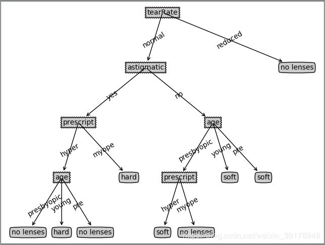
我们可以看到,其实创建好分类器后,在面对实际问题的时候,最重要的一步无非就是将数据集处理成我们想要的格式,并与分类器的输入匹配。从上图我们可以看出,医生最多需要问四个问题就能够确认患者需要佩戴的隐形眼镜类型。
(7)本章小结
这一章节我们主要学习的是决策树中的ID3算法,ID3名字中的ID指的是Iterative Dichotomiser(迭代二分器),这是一个很好的算法,但是它也存在很多问题,它是基于“信息增益最大化”来进行的,在许多场合下不免暴露其“贪心”本质。
上面案例中的决策树非常好地匹配了实验数据,但是这些匹配选项可能太多了,我们将这种问题称之为过度匹配(overfitting)。
我们后期可能需要学习预剪枝、后剪枝等操作,来优化我们的算法。另外在西瓜书上除了剪枝操作已经非常详细地作了介绍,还为我们展示了包括连续值、缺失值的处理方法。本章介绍的主要还是针对离散属性。
3 完整代码
以下是trees.py完整代码:
'''
Created on Oct 12, 2010
Decision Tree Source Code for Machine Learning in Action Ch. 3
@author: Peter Harrington
'''
from math import log
import operator

#生成数据集
def createDataSet():
    dataSet = [[1, 1, 'yes'],
               [1, 1, 'yes'],
               [1, 0, 'no'],
               [0, 1, 'no'],
               [0, 1, 'no']]
    labels = ['no surfacing','flippers']
    #change to discrete values
    return dataSet, labels

#计算指定数据集的香农熵
def calcShannonEnt(dataSet):
    numEntries = len(dataSet)#获取数据集样本个数
    labelCounts = {}#初始化一个字典用来保存每个标签出现的次数
    for featVec in dataSet:
        currentLabel = featVec[-1]#逐个获取标签信息
        # 如果标签没有放入统计次数字典的话,就添加进去
        if currentLabel not in labelCounts.keys(): labelCounts[currentLabel] = 0
        labelCounts[currentLabel] += 1
    shannonEnt = 0.0#初始化香农熵
    for key in labelCounts:
        prob = float(labelCounts[key])/numEntries#选择该标签的概率
        shannonEnt -= prob * log(prob,2)#公式计算
    return shannonEnt

#划分数据集
def splitDataSet(dataSet, axis, value):
    retDataSet = []#创建新列表以存放满足要求的样本
    for featVec in dataSet:
        if featVec[axis] == value:
            # 下面这两句用来将axis特征去掉,并将符合条件的添加到返回的数据集中
            reducedFeatVec = featVec[:axis]
            reducedFeatVec.extend(featVec[axis+1:])
            retDataSet.append(reducedFeatVec)
    return retDataSet

#选择最好的数据集划分方式
def chooseBestFeatureToSplit(dataSet):
    numFeatures = len(dataSet[0]) - 1#获取样本集中特征个数,-1是因为最后一列是label
    baseEntropy = calcShannonEnt(dataSet)#计算根节点的信息熵
    bestInfoGain = 0.0#初始化信息增益
    bestFeature = -1#初始化最优特征的索引值
    for i in range(numFeatures):#遍历所有特征,i表示第几个特征
        featList = [example[i] for example in dataSet]#将dataSet中的数据按行依次放入example中,然后取得example中的example[i]元素,即获得特征i的所有取值
        uniqueVals = set(featList)#由上一步得到了特征i的取值,比如[1,1,1,0,0],使用集合这个数据类型删除多余重复的取值,则剩下[1,0]
        newEntropy = 0.0
        for value in uniqueVals:
            subDataSet = splitDataSet(dataSet, i, value)#逐个划分数据集,得到基于特征i和对应的取值划分后的子集
            prob = len(subDataSet)/float(len(dataSet))#根据特征i可能取值划分出来的子集的概率
            newEntropy += prob * calcShannonEnt(subDataSet)#求解分支节点的信息熵
        infoGain = baseEntropy - newEntropy#计算信息增益
        if (infoGain > bestInfoGain): #对循环求得的信息增益进行大小比较
            bestInfoGain = infoGain
            bestFeature = i#如果计算所得信息增益最大,则求得最佳划分方法
    return bestFeature#返回划分属性(特征)

#多数表决函数
def majorityCnt(classList):
    classCount={}
    for vote in classList:
        if vote not in classCount.keys(): classCount[vote] = 0
        classCount[vote] += 1
    # 分解为元组列表,operator.itemgetter(1)按照第二个元素的次序对元组进行排序,reverse=True是逆序,即按照从大到小的顺序排列
    sortedClassCount = sorted(classCount.iteritems(), key=operator.itemgetter(1), reverse=True)
    return sortedClassCount[0][0]

#构建决策树
def createTree(dataSet,labels):
    classList = [example[-1] for example in dataSet]#获取类别标签
    if classList.count(classList[0]) == len(classList):
        return classList[0]#类别完全相同则停止继续划分
    if len(dataSet[0]) == 1:
        return majorityCnt(classList)#遍历完所有特征时返回出现次数最多的类别
    bestFeat = chooseBestFeatureToSplit(dataSet)#选取最优划分特征
    bestFeatLabel = labels[bestFeat]#获取最优划分特征对应的属性标签
    myTree = {bestFeatLabel:{}}#存储树的所有信息
    del(labels[bestFeat])#删除已经使用过的属性标签
    featValues = [example[bestFeat] for example in dataSet]#得到训练集中所有最优特征的属性值
    uniqueVals = set(featValues)#去掉重复的属性值
    for value in uniqueVals:#遍历特征,创建决策树
        subLabels = labels[:]#剩余的属性标签列表
        myTree[bestFeatLabel][value] = createTree(splitDataSet(dataSet, bestFeat, value),subLabels)#递归函数实现决策树的构建
    return myTree

#决策树分类器
def classify(inputTree,featLabels,testVec):
    firstStr = list(inputTree.keys())[0]#获取根节点
    secondDict = inputTree[firstStr]#获取下一级分支
    featIndex = featLabels.index(firstStr)#查找当前列表中第一个匹配firstStr变量的元素的索引
    key = testVec[featIndex]#获取测试样本中,与根节点特征对应的取值
    valueOfFeat = secondDict[key]#获取测试样本通过第一个特征分类器后的输出
    if isinstance(valueOfFeat, dict): # 判断节点是否为字典来以此判断是否为叶节点
        classLabel = classify(valueOfFeat, featLabels, testVec)
    else: classLabel = valueOfFeat#如果到达叶子节点,则返回当前节点的分类标签
    return classLabel

#序列化对象
def storeTree(inputTree, filename):
    import pickle
    fw = open(filename, 'wb+')  # 读写方式建立一个二进制文件
    pickle.dump(inputTree, fw)  # 把对象序列化后写入文件
    fw.close()

#反序列化
def grabTree(filename):
    import pickle
    fr = open(filename, 'rb')
    return pickle.load(fr)  # 反序列化对象,返回数据类型与存储前一致
以下是treePlotter.py完整代码:
'''
Created on Oct 14, 2010

@author: Peter Harrington
'''
import matplotlib.pyplot as plt

decisionNode = dict(boxstyle="sawtooth", fc="0.8")
leafNode = dict(boxstyle="round4", fc="0.8")
arrow_args = dict(arrowstyle="<-")

def getNumLeafs(myTree):
    numLeafs = 0
    firstStr = list(myTree.keys())[0]
    secondDict = myTree[firstStr]
    for key in secondDict.keys():
        if type(secondDict[key]).__name__=='dict':#test to see if the nodes are dictonaires, if not they are leaf nodes
            numLeafs += getNumLeafs(secondDict[key])
        else:   numLeafs +=1
    return numLeafs

def getTreeDepth(myTree):
    maxDepth = 0
    firstStr = list(myTree.keys())[0]
    secondDict = myTree[firstStr]
    for key in secondDict.keys():
        if type(secondDict[key]).__name__=='dict':#test to see if the nodes are dictonaires, if not they are leaf nodes
            thisDepth = 1 + getTreeDepth(secondDict[key])
        else:   thisDepth = 1
        if thisDepth > maxDepth: maxDepth = thisDepth
    return maxDepth

def plotNode(nodeTxt, centerPt, parentPt, nodeType):
    createPlot.ax1.annotate(nodeTxt, xy=parentPt,  xycoords='axes fraction',
             xytext=centerPt, textcoords='axes fraction',
             va="center", ha="center", bbox=nodeType, arrowprops=arrow_args )

def plotMidText(cntrPt, parentPt, txtString):
    xMid = (parentPt[0]-cntrPt[0])/2.0 + cntrPt[0]
    yMid = (parentPt[1]-cntrPt[1])/2.0 + cntrPt[1]
    createPlot.ax1.text(xMid, yMid, txtString, va="center", ha="center", rotation=30)

def plotTree(myTree, parentPt, nodeTxt):#if the first key tells you what feat was split on
    numLeafs = getNumLeafs(myTree)  #this determines the x width of this tree
    depth = getTreeDepth(myTree)
    firstStr = list(myTree.keys())[0]     #the text label for this node should be this
    cntrPt = (plotTree.xOff + (1.0 + float(numLeafs))/2.0/plotTree.totalW, plotTree.yOff)
    plotMidText(cntrPt, parentPt, nodeTxt)
    plotNode(firstStr, cntrPt, parentPt, decisionNode)
    secondDict = myTree[firstStr]
    plotTree.yOff = plotTree.yOff - 1.0/plotTree.totalD
    for key in secondDict.keys():
        if type(secondDict[key]).__name__=='dict':#test to see if the nodes are dictonaires, if not they are leaf nodes
            plotTree(secondDict[key],cntrPt,str(key))        #recursion
        else:   #it's a leaf node print the leaf node
            plotTree.xOff = plotTree.xOff + 1.0/plotTree.totalW
            plotNode(secondDict[key], (plotTree.xOff, plotTree.yOff), cntrPt, leafNode)
            plotMidText((plotTree.xOff, plotTree.yOff), cntrPt, str(key))
    plotTree.yOff = plotTree.yOff + 1.0/plotTree.totalD
#if you do get a dictonary you know it's a tree, and the first element will be another dict

def createPlot(inTree):
    fig = plt.figure(1, facecolor='white')
    fig.clf()
    axprops = dict(xticks=[], yticks=[])
    createPlot.ax1 = plt.subplot(111, frameon=False, **axprops)    #no ticks
    #createPlot.ax1 = plt.subplot(111, frameon=False) #ticks for demo puropses
    plotTree.totalW = float(getNumLeafs(inTree))
    plotTree.totalD = float(getTreeDepth(inTree))
    plotTree.xOff = -0.5/plotTree.totalW; plotTree.yOff = 1.0;
    plotTree(inTree, (0.5,1.0), '')
    plt.show()

#def createPlot():
#    fig = plt.figure(1, facecolor='white')
#    fig.clf()
#    createPlot.ax1 = plt.subplot(111, frameon=False) #ticks for demo puropses
#    plotNode('a decision node', (0.5, 0.1), (0.1, 0.5), decisionNode)
#    plotNode('a leaf node', (0.8, 0.1), (0.3, 0.8), leafNode)
#    plt.show()

def retrieveTree(i):
    listOfTrees =[{'no surfacing': {0: 'no', 1: {'flippers': {0: 'no', 1: 'yes'}}}},
                  {'no surfacing': {0: 'no', 1: {'flippers': {0: {'head': {0: 'no', 1: 'yes'}}, 1: 'no'}}}}
                  ]
    return listOfTrees[i]

#createPlot(thisTree)