人工智能实践：Tensorflow笔记（2）——神经网络优化

1、预备知识

tf.where()
条件语句真返回A，条件语句假返回B

tf.where(条件语句,真返回A,假返回B)

import tensorflow as tf

a = tf.constant([1,2,3,1,1])
b = tf.constant([0,1,3,4,5])
c = tf.where(tf.greater(a,b),a,b)       #若a>b，返回a对应位置的元素，否则返回b对应位置的元素
print("c:",c)

np.random.RandomState.rand()
返回一个[0,1)之间的随机数

np.random.RandomState.rand(维度)		#维度为空，返回标量

import numpy as np

rdm = np.random.RandomState(seed=1)     #seed=常数每次生成随机数相同
a = rdm.rand()          #返回一个随机标量
b = rdm.rand(2,3)       #返回维度为2行3列随机数矩阵
print("a:",a)
print("b:",b)

运行结果：

np.vstack
将两个数组按垂直方向叠加

np.vstack(数组1,数组2)

import numpy as np

a = np.array([1,2,3])
b = np.array([4,5,6])
c = np.vstack((a,b))
print("c:\n",c)

np.mgrid[ ] .ravel() np.c_[ ] 生成网格坐标点

• np.mgrid[ ] [起始值 结束值)

np.mgrid[起始值：结束值：步长，起始值：结束值：步长，...]

• x.ravel() 将x变为一维数组，“把.前变量拉直”
• np.c_[ ] 使返回的间隔数值点配对

np.c_[数组1，数组2，...]

import numpy as np

x,y = np.mgrid[1:3:1,2:4:0.5]
grid = np.c_[x.ravel(),y.ravel()]
print("x:",x)
print("y:",y)
print("grid:\n",grid)

2、神经网络（NN）复杂度

• NN复杂度：多用NN层数和NN参数的个数表示
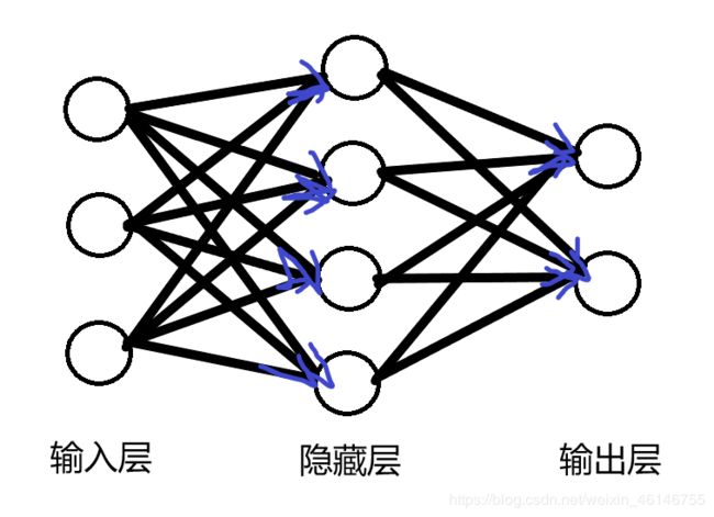
  空间复杂度：
  层数=隐藏层的层数+1个输出层（如图为2层NN）
  总参数=总w+总b（如图3 * 4+4（第1层）+4 * 2+2（第2层）=26）
  时间复杂度：
  乘加运算次数：（如图3 * 4（第1层）+4 * 2（第2层）=20）

• 指数衰减学习率
  可以先用较大的学习率，快速得到较优解，然后逐步减小学习率，使模型在训练后期稳定。
  指数衰减学习率=初始学习率*学习率衰减率（当前轮数/多少轮衰减一次）

epoch = 40
LR_BASE = 0.2
LR_DECAY = 0.99
LR_STEP = 1

for epoch in range(epoch):
    lr = LR_BASE * LR_DECAY ** (epoch / LR_STEP)
    with tf.GradientTape() as tape:
        loss = tf.square(w+1)
    grads = tape.gradient(loss,w)

    w.assign_sub(lr * grads)
    print("After %s epoch,w is %f,loss is %f,lr is %f" %(epoch,w.numpy(),loss,lr))

3、激活函数

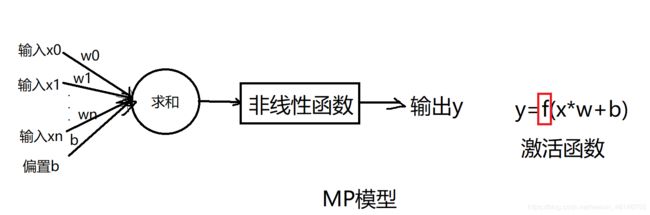
激活函数的加入提升了模型的表达力，使得多层神经网络不再是输入x的线性组合

• 优秀的激活函数：
  非线性：激活函数非线性时，多层神经网络可逼近所有函数（只有当激活函数是非线性时，才不会被单层网络所替代，使多层网络有了意义）
  可微性：优化器大多用梯度下降更新参数（如果激活函数不可微，就无法更新参数）
  单调性：当激活函数是单调的，能保证单层网络的损失函数是凸函数（更容易收敛）
  近似恒等性：f(x)约等于x当参数初始化为随机小值时，神经网络更稳定
• 激活函数输出值的范围：
  激活函数输出为有限值时，基于梯度的优化方法更稳定（因为权重对特征的影响更显著一些）
  激活函数输出为无限值时，建议调小学习率（因为参数的初始值对模型的影响很大）

常用激活函数
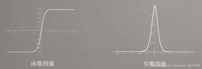
Sigmoid函数

tf.nn.sigmoid(x)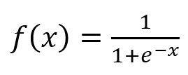

特点：
（1）易造成梯度消失（深层神经网络更新参数时，需要从输出层到输入层进行链式求导，而sigmoid函数的导数输出是0到0.25间的小数，链式求导需要多层导数连续相乘，会出现多个0到0.25之间的连续相乘，结果将趋于0，产生梯度消失，使得参数无法继续更新）
（2）输出非0均值，收敛慢
（3）幂运算复杂，训练时间长
Tanh函数

tf.math.tanh(x）

特点：
（1）输出是0均值
（2）易造成梯度消失
（3）幂运算复杂，训练时间长

Relu函数

tf.nn.relu(x)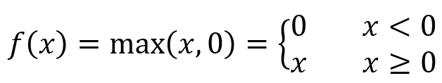

优点：
（1）解决了梯度消失问题（在正区间）
（2）只需判断输入是否大于0，计算速度快
（3）收敛速度远快于sigmoid和tanh
缺点：
（1）输出非0均值，收敛慢
（2）Dead Relu问题：某些神经元可能永远不被激活，导致相应的参数永远不能被更新（送入激活函数的输入特征是负数时，激活函数输出是0，反向传播得到的梯度是0）

造成神经元死亡的根本原因：经过relu函数的负数特征过多导致，可以通过改进随机初始化，避免过多的负数特征送入relu函数，通过设置更小的学习率，减少参数分布的巨大变化，避免训练中产生过多负数特征进入relu函数

Leaky Relu函数

tf.nn.leaky_relu(x)

理论上来讲，Leaky Relu有Relu的所有优点，外加不会有Dead Relu问题，但是在实际操作中，并没有完全证明Leaky Relu总是好于Relu

对于初学者选择激活函数：
首选relu激活函数
学习率设置较小值
输入特征标准化，即让输入特征满足以0为均值，1为标准差的正态分布
初始参数中心化，即让随机生成的参数满足以0为均值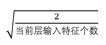，为标准差的正态分布

4、损失函数

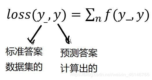
• 损失函数（loss）：预测值（y）与已知答案（y_）的差距
  
• 均方误差mse：
  

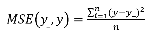
loss_mse = tf.reduce_mean(tf.square(y_-y))

预测酸奶日销量y，x1、x2是影响日销量的因素。
建模前，应预先采集的数据有：每日x1、x2和销量y_（即已知答案，最佳情况：产量=销量）
拟造数据集X，Y_：y_=x1+x2 噪声：-0.05~+0.05 拟合可以预测销量的函数

import tensorflow as tf
import numpy as np

SEED = 23455

rdm = np.random.RandomState(seed=SEED)      #生成[0，1）之间的随机数
x = rdm.rand(32,2)
y_ = [[x1 + x2 + (rdm.rand() / 10.0 - 0.05)] for (x1,x2) in x]      #生成噪声[0,1)/10=[0,0.1);
x = tf.cast(x,dtype=tf.float32)

w1 = tf.Variable(tf.random.normal([2,1],stddev=1,seed=1))

epoch = 15000
lr = 0.002

for epoch in range(epoch):
    with tf.GradientTape() as tape:
        y = tf.matmul(x,w1)
        loss_mse = tf.square(y_-y)

    grads = tape.gradient(loss_mse,w1)
    w1.assign_sub(lr * grads)

    if epoch % 500 == 0:
        print("After %d training steps,w1 is " %(epoch))
        print(w1.numpy(),"\n")
print("Final w1 is: ",w1.numpy())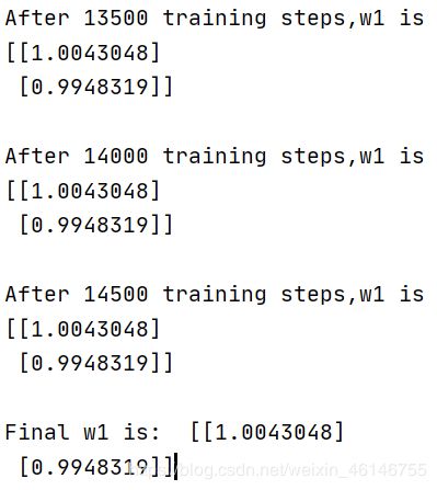

可以看出两个参数正向1趋近，最后得到神经网络的参数是接近1的，拟合出的预测销量y的结果y=1.00 * x1+0.99 * x2，该结果和制造数据集公式y=1 * x1+1 * x2一致，说明预测酸奶日销量的公式拟合正确

• 自定义损失函数
  如预测产品销量，预测多了，损失成本；预测少了，损失利润。
  若利润不等于成本，则mse产生的loss无法利益最大化

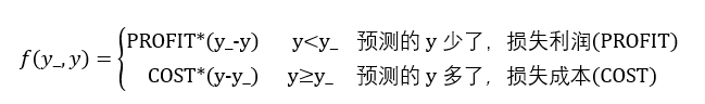
如：预测酸奶销量，酸奶成本（COST）1元，酸奶利润（PROFIT）99元。
预测少了损失利润99元，预测多了损失成本1元。
预测少了损失大，希望生成的预测函数往多了预测。

import tensorflow as tf
import numpy as np

SEED = 23455
COST = 1
PROFIT = 99

rdm = np.random.RandomState(SEED)
x = rdm.rand(32, 2)
y_ = [[x1 + x2 + (rdm.rand() / 10.0 - 0.05)] for (x1, x2) in x]  # 生成噪声[0,1)/10=[0,0.1); [0,0.1)-0.05=[-0.05,0.05)
x = tf.cast(x, dtype=tf.float32)

w1 = tf.Variable(tf.random.normal([2, 1], stddev=1, seed=1))

epoch = 10000
lr = 0.002

for epoch in range(epoch):
    with tf.GradientTape() as tape:
        y = tf.matmul(x, w1)
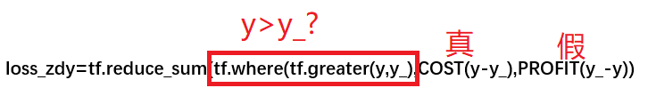
        loss = tf.reduce_sum(tf.where(tf.greater(y, y_), (y - y_) * COST, (y_ - y) * PROFIT))

    grads = tape.gradient(loss, w1)
    w1.assign_sub(lr * grads)

    if epoch % 500 == 0:
        print("After %d training steps,w1 is " % (epoch))
        print(w1.numpy(), "\n")
print("Final w1 is: ", w1.numpy())

# 自定义损失函数
# 酸奶成本1元， 酸奶利润99元
# 成本很低，利润很高，人们希望多预测些，生成模型系数大于1，往多了预测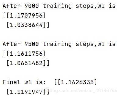

• 交叉熵损失函数CE（Cross Entropy）：表征两个概率分布之间的距离
  
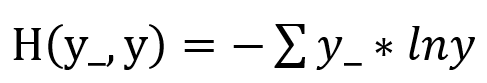
  交叉熵越大，两个概率分布越远；交叉熵越小，两个概率分布越近。

eg.二分类
已知答案y_=(1,0)，预测y1=(0.6,0.4)，y2=(0.8,0.2)，哪个更接近标准答案？

因为H1>H2，所以y2预测 更准

tf.losses.categorical_crossentropy(y_,y)

import tensorflow as tf

loss_ce1 = tf.losses.categorical_crossentropy([1,0],[0.6,0.4])
loss_ce2 = tf.losses.categorical_crossentropy([1,0],[0.8,0.2])
print("loss_ce1:",loss_ce1)
print("loss_ce2:",loss_ce2)

• softmax与交叉熵结合
  输出先过softmax函数，再计算y与y_的交叉熵损失函数。

tf.nn.softmax_cross_entropy_with_logits(y_,y)

import tensorflow as tf
import numpy as  np

y_ = np.array([[1,0,0],[0,1,0],[0,0,1],[1,0,0],[0,1,0]])
y = np.array([[12,3,2],[3,10,1],[1,2,5],[4,6.5,1.2],[3,6,1]])
y_pro = tf.nn.softmax(y)
loss_ce1 = tf.losses.categorical_crossentropy(y_,y_pro)
loss_ce2 = tf.nn.softmax_cross_entropy_with_logits(y_,y)

print('分步计算的结果：\n',loss_ce1)
print('结合计算的结果：\n',loss_ce2)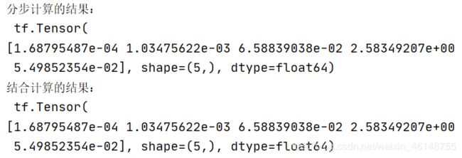

5、缓解过拟合

欠拟合和过拟合
欠拟合是模型不能有效拟合数据集，是对现有数据集学习得不够彻底
过拟合是模型对当前数据拟合得太好了，但对未见过的新数据无法做出准确判断，模型缺乏泛化力

• 欠拟合的解决方法：
  增加输入特征项
  增加网络参数
  减少正则化参数
• 过拟合的解决方法：
  数据清洗
  增大训练集
  采用正则化
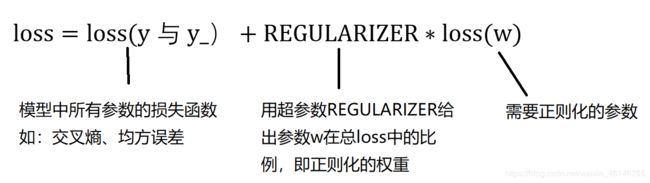
  增大正则化参数
• 正则化缓解过拟合
  正则化在损失函数中引入模型复杂度指标，利用给W加权值，弱化了训练数据的噪声（一般不正则化b）
  
  
  
• 正则化的选择
  L1正则化大概率会使很多参数变为零，因此该方法可通过稀疏参数，即减少参数的数量，降低复杂度
  L2正则化会使参数很接近零但不为零，因此该方法可通过减少参数值的大小降低复杂度

# 导入所需模块
import tensorflow as tf
from matplotlib import pyplot as plt
import numpy as np
import pandas as pd

# 读入数据/标签 生成x_train y_train
df = pd.read_csv('dot.csv')
x_data = np.array(df[['x1', 'x2']])
y_data = np.array(df['y_c'])

x_train = np.vstack(x_data).reshape(-1,2)
y_train = np.vstack(y_data).reshape(-1,1)

Y_c = [['red' if y else 'blue'] for y in y_train]

# 转换x的数据类型，否则后面矩阵相乘时会因数据类型问题报错
x_train = tf.cast(x_train, tf.float32)
y_train = tf.cast(y_train, tf.float32)

# from_tensor_slices函数切分传入的张量的第一个维度，生成相应的数据集，使输入特征和标签值一一对应
train_db = tf.data.Dataset.from_tensor_slices((x_train, y_train)).batch(32)

# 生成神经网络的参数，输入层为2个神经元，隐藏层为11个神经元，1层隐藏层，输出层为1个神经元
# 用tf.Variable()保证参数可训练
w1 = tf.Variable(tf.random.normal([2, 11]), dtype=tf.float32)
b1 = tf.Variable(tf.constant(0.01, shape=[11]))

w2 = tf.Variable(tf.random.normal([11, 1]), dtype=tf.float32)
b2 = tf.Variable(tf.constant(0.01, shape=[1]))

lr = 0.01  # 学习率
epoch = 400  # 循环轮数

# 训练部分
for epoch in range(epoch):
    for step, (x_train, y_train) in enumerate(train_db):
        with tf.GradientTape() as tape:  # 记录梯度信息

            h1 = tf.matmul(x_train, w1) + b1  # 记录神经网络乘加运算
            h1 = tf.nn.relu(h1)
            y = tf.matmul(h1, w2) + b2

            # 采用均方误差损失函数mse = mean(sum(y-out)^2)
            loss = tf.reduce_mean(tf.square(y_train - y))

        # 计算loss对各个参数的梯度
        variables = [w1, b1, w2, b2]
        grads = tape.gradient(loss, variables)

        # 实现梯度更新
        # w1 = w1 - lr * w1_grad tape.gradient是自动求导结果与[w1, b1, w2, b2] 索引为0，1，2，3 
        w1.assign_sub(lr * grads[0])
        b1.assign_sub(lr * grads[1])
        w2.assign_sub(lr * grads[2])
        b2.assign_sub(lr * grads[3])

    # 每20个epoch，打印loss信息
    if epoch % 20 == 0:
        print('epoch:', epoch, 'loss:', float(loss))

# 预测部分
print("*******predict*******")
# xx在-3到3之间以步长为0.01，yy在-3到3之间以步长0.01,生成间隔数值点
xx, yy = np.mgrid[-3:3:.1, -3:3:.1]
# 将xx , yy拉直，并合并配对为二维张量，生成二维坐标点
grid = np.c_[xx.ravel(), yy.ravel()]
grid = tf.cast(grid, tf.float32)
# 将网格坐标点喂入神经网络，进行预测，probs为输出
probs = []
for x_test in grid:
    # 使用训练好的参数进行预测
    h1 = tf.matmul([x_test], w1) + b1
    h1 = tf.nn.relu(h1)
    y = tf.matmul(h1, w2) + b2  # y为预测结果
    probs.append(y)

# 取第0列给x1，取第1列给x2
x1 = x_data[:, 0]
x2 = x_data[:, 1]
# probs的shape调整成xx的样子
probs = np.array(probs).reshape(xx.shape)
plt.scatter(x1, x2, color=np.squeeze(Y_c)) #squeeze去掉纬度是1的纬度,相当于去掉[['red'],[''blue]],内层括号变为['red','blue']
# 把坐标xx yy和对应的值probs放入contour<[‘kɑntʊr]>函数，给probs值为0.5的所有点上色  plt点show后 显示的是红蓝点的分界线
plt.contour(xx, yy, probs, levels=[.5])
plt.show()

# 读入红蓝点，画出分割线，不包含正则化
# 不清楚的数据，建议print出来查看 

加入L2正则化

# 导入所需模块
import tensorflow as tf
from matplotlib import pyplot as plt
import numpy as np
import pandas as pd

# 读入数据/标签 生成x_train y_train
df = pd.read_csv('dot.csv')
x_data = np.array(df[['x1', 'x2']])
y_data = np.array(df['y_c'])

x_train = x_data
y_train = y_data.reshape(-1, 1)

Y_c = [['red' if y else 'blue'] for y in y_train]

# 转换x的数据类型，否则后面矩阵相乘时会因数据类型问题报错
x_train = tf.cast(x_train, tf.float32)
y_train = tf.cast(y_train, tf.float32)

# from_tensor_slices函数切分传入的张量的第一个维度，生成相应的数据集，使输入特征和标签值一一对应
train_db = tf.data.Dataset.from_tensor_slices((x_train, y_train)).batch(32)

# 生成神经网络的参数，输入层为4个神经元，隐藏层为32个神经元，2层隐藏层，输出层为3个神经元
# 用tf.Variable()保证参数可训练
w1 = tf.Variable(tf.random.normal([2, 11]), dtype=tf.float32)
b1 = tf.Variable(tf.constant(0.01, shape=[11]))

w2 = tf.Variable(tf.random.normal([11, 1]), dtype=tf.float32)
b2 = tf.Variable(tf.constant(0.01, shape=[1]))

lr = 0.01  # 学习率为
epoch = 400  # 循环轮数

# 训练部分
for epoch in range(epoch):
    for step, (x_train, y_train) in enumerate(train_db):
        with tf.GradientTape() as tape:  # 记录梯度信息

            h1 = tf.matmul(x_train, w1) + b1  # 记录神经网络乘加运算
            h1 = tf.nn.relu(h1)
            y = tf.matmul(h1, w2) + b2

            # 采用均方误差损失函数mse = mean(sum(y-out)^2)
            loss_mse = tf.reduce_mean(tf.square(y_train - y))
            # 添加l2正则化
            loss_regularization = []
            # tf.nn.l2_loss(w)=sum(w ** 2) / 2
            loss_regularization.append(tf.nn.l2_loss(w1))
            loss_regularization.append(tf.nn.l2_loss(w2))
            # 求和
            # 例：x=tf.constant(([1,1,1],[1,1,1]))
            #   tf.reduce_sum(x)
            # >>>6
            # loss_regularization = tf.reduce_sum(tf.stack(loss_regularization))
            loss_regularization = tf.reduce_sum(loss_regularization)
            loss = loss_mse + 0.03 * loss_regularization #REGULARIZER = 0.03

        # 计算loss对各个参数的梯度
        variables = [w1, b1, w2, b2]
        grads = tape.gradient(loss, variables)

        # 实现梯度更新
        # w1 = w1 - lr * w1_grad
        w1.assign_sub(lr * grads[0])
        b1.assign_sub(lr * grads[1])
        w2.assign_sub(lr * grads[2])
        b2.assign_sub(lr * grads[3])

    # 每200个epoch，打印loss信息
    if epoch % 20 == 0:
        print('epoch:', epoch, 'loss:', float(loss))

# 预测部分
print("*******predict*******")
# xx在-3到3之间以步长为0.01，yy在-3到3之间以步长0.01,生成间隔数值点
xx, yy = np.mgrid[-3:3:.1, -3:3:.1]
# 将xx, yy拉直，并合并配对为二维张量，生成二维坐标点
grid = np.c_[xx.ravel(), yy.ravel()]
grid = tf.cast(grid, tf.float32)
# 将网格坐标点喂入神经网络，进行预测，probs为输出
probs = []
for x_predict in grid:
    # 使用训练好的参数进行预测
    h1 = tf.matmul([x_predict], w1) + b1
    h1 = tf.nn.relu(h1)
    y = tf.matmul(h1, w2) + b2  # y为预测结果
    probs.append(y)

# 取第0列给x1，取第1列给x2
x1 = x_data[:, 0]
x2 = x_data[:, 1]
# probs的shape调整成xx的样子
probs = np.array(probs).reshape(xx.shape)
plt.scatter(x1, x2, color=np.squeeze(Y_c))
# 把坐标xx yy和对应的值probs放入contour<[‘kɑntʊr]>函数，给probs值为0.5的所有点上色  plt点show后 显示的是红蓝点的分界线
plt.contour(xx, yy, probs, levels=[.5])
plt.show()

# 读入红蓝点，画出分割线，包含正则化
# 不清楚的数据，建议print出来查看 

加入L2正则化后的曲线更平缓，有效缓解了过拟合

6、优化器

神经网络优化器
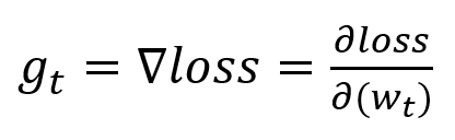
待优化参数w，损失函数loss，学习率lr，每次迭代一个batch，t表示当前batch迭代的总次数：

1. 计算t时刻损失函数关于当前参数的梯度
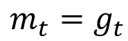
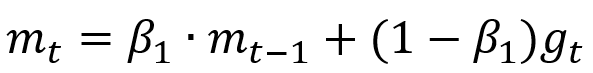
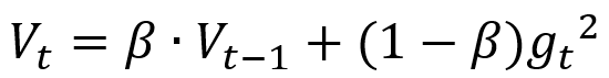
2. 计算t时刻一阶动量和二阶动量
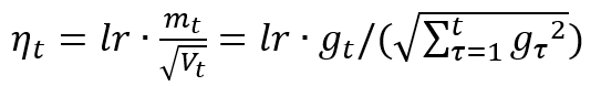
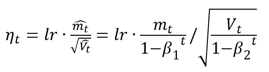
3. 计算t时刻下降梯度：
   
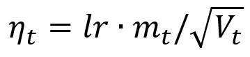
4. 计算t+1时刻参数：
   
   一阶动量：与梯度相关的函数
   二阶动量：与梯度平方相关的函数

优化器
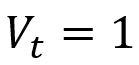
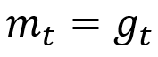
SGD(无momentum) 常用的梯度下降法

w1.assign_sub(lr*grads[0])
b1.assign_sub(lr*grads[1])

SGDM(含momentum的SGD) 在SGD基础上增加一阶动量

m_w,m_b = 0,0
beta = 0.9

m_w = beta * m_w + (1 - beta) * grads[0]
m_b = beta * m_b + (1 - beta) * grads[1]
w1.assign_sub(lr * m_w)
b1.assign_sub(lr * m_b)

Adagrad 在SGD基础上增加二阶动量

v_w,v_b = 0,0
v_w += tf.square(grads[0])
v_b += tf.square(grads[1])
w1.assign_sub(lr * grads[0] / tf.sqrt(v_w))
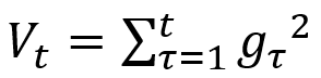
b1.assign_sub(lr * grads[1] / tf.sqrt(v_b))

RMSProp SGD基础上增加二阶动量

v_w,v_b = 0,0
beta = 0.9
v_w = beta * v_w + (1 - beta) * tf.square(grads[0])
v_b = beta * v_b + (1 - beta) * tf.square(grads[1])
w1.assign_sub(lr * grads[0] / tf.sqrt(v_w))
b1.assign_sub(lr * grads[1] / tf.sqrt(v_b))

Adam 同时结合SGDM一阶动量和RMSProp二阶动量

修正一阶动量的偏差：


修正二阶动量的偏差：

m_w, m_b = 0, 0
v_w, v_b = 0, 0
beta1, beta2 = 0.9, 0.999
delta_w, delta_b = 0, 0
global_step = 0

m_w = beta1 * m_w + (1 - beta1) * grads[0]
m_b = beta1 * m_b + (1 - beta1) * grads[1]
v_w = beta2 * v_w + (1 - beta2) * tf.square(grads[0])
v_b = beta2 * v_b + (1 - beta2) * tf.square(grads[1])

m_w_correction = m_w / (1 - tf.pow(beta1, int(global_step)))
m_b_correction = m_b / (1 - tf.pow(beta1, int(global_step)))
v_w_correction = v_w / (1 - tf.pow(beta2, int(global_step)))
v_b_correction = v_b / (1 - tf.pow(beta2, int(global_step)))

w1.assign_sub(lr * m_w_correction / tf.sqrt(v_w_correction))
b1.assign_sub(lr * m_b_correction / tf.sqrt(v_b_correction))