菜鸟笔记-DuReader阅读理解基线模型代码阅读笔记（六）—— 模型构建

系列目录：

1. 菜鸟笔记-DuReader阅读理解基线模型代码阅读笔记（一）——
   数据
2. 菜鸟笔记-DuReader阅读理解基线模型代码阅读笔记（二）——
   介绍及分词
3. 菜鸟笔记-DuReader阅读理解基线模型代码阅读笔记（三）—— 预处理
4. 菜鸟笔记-DuReader阅读理解基线模型代码阅读笔记（四）—— 段落抽取
5. 菜鸟笔记-DuReader阅读理解基线模型代码阅读笔记（五）—— 准备数据
   未完待续 … …
   基线系统使用RCModel类实现了阅读理解模型，具体代码见/tensorflow/rc_model.py。系统实现了BiDAF 和Match-LSTM两个模型，可以通过设置参数–algo 进行切换，下面对模型进行简单介绍。

QA模型的通用结构

基线系统是从原文中寻找答案，属于抽取式问答模型。模型的输入为[文档，问题]，输出是[答案起始索引，答案终止索引]∈ [ 0, len(文档) ]。两个模型都属于神经网络阅读理解模型，其基本框架主要包括词汇嵌入层（Word-Embedder）、编码层（Encoder）、文档-问题交互层（Interaction-Layer）、作答层（Answer Layer）。如下图所示：

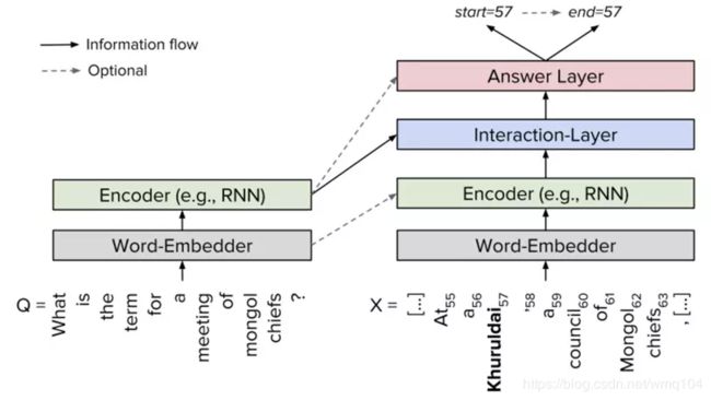
其中，词嵌入层负责将文档和问题中的词语映射为语义特征向量表示；编码层使用循环神经网络（RNN）来对文档和问题进行编码，编码后每个词语的语义特征向量会包含上下文的语义信息；文档-问题交互层主要负责捕捉问题和文档的相关关系，并输出融合了问题-文档语义信息的特征矩阵；最后作答层基于相关特征矩阵预测答案的具体范围。
Match-LSTM与 BiDAF 模型的区别主要是在文档-问题交互层，他们一个采用了Match-LSTM层、一个采用了Attention Flow层，具体实现如下。

整体计算图构建

构建计算图在_build_graph函数中实现，源代码见/tensorflow/rc_model.py

def _build_graph(self):
     """
     使用Tensorflow构建计算图
     """
     start_t = time.time()
     self._setup_placeholders() #占位符，用于输入变量
     self._embed()  #嵌入层
     self._encode() #编码层、使用两个Bi-LSTM层分别对文档和问题进行编码
     self._match() #文档-问题交互层，RC模型的核心，通过BIDAF或MLSTM获得问题相关的文档编码
     self._fuse() #在交互层之后再次使用Bi-LSTM将问题相关的上下文信息进行融合
     self._decode()# 使用Pointer网络获取每个位置是预测答案起始或终止位置的概率。
     self._compute_loss()#计算模型输出误差
     self._create_train_op()#创建训练操作
     self.logger.info('Time to build graph: {} s'.format(time.time() - start_t))
     param_num = sum([np.prod(self.sess.run(tf.shape(v))) for v in self.all_params])
     self.logger.info('There are {} parameters in the model'.format(param_num))

有代码可知，模型主要包括嵌入层、编码层、文档-问题交互层、上下文信息融合层、解答层。

关键层实现

编码层

    def _encode(self):
        """
        使用两个Bi-LSTM层分别对文档和问题进行编码
        """
        with tf.variable_scope('passage_encoding'):
            self.sep_p_encodes, _ = rnn('bi-lstm', self.p_emb, self.p_length, self.hidden_size)
        with tf.variable_scope('question_encoding'):
            self.sep_q_encodes, _ = rnn('bi-lstm', self.q_emb, self.q_length, self.hidden_size)
        if self.use_dropout:
            self.sep_p_encodes = tf.nn.dropout(self.sep_p_encodes, self.dropout_keep_prob)
            self.sep_q_encodes = tf.nn.dropout(self.sep_q_encodes, self.dropout_keep_prob)

代码在rnn('bi-lstm', self.p_emb, self.p_length, self.hidden_size)中实现了(Bi-)LSTM, (Bi-)GRU and (Bi-)RNN，这个函数输入输出为：

输入:
    rnn_type: rnn的种类
    inputs: 填充后的输入
    length: 输入的有效长度
    hidden_size: 隐藏层的大小
    layer_num: 堆叠的rnn层数量
    dropout_keep_prob: dropout比例
    concat: 布尔变量，如果rnn是双向，当为真时两个方向的向量拼接后输出，为假时加和后输出
输出:
    RNN 的输出
    RNN的最终状态

文档-问题交互层（_match）

文档-问题交互层，RC模型的核心，通过BIDAF或MLSTM获得问题相关的文档编码。

MLSTM

MatchLSTMAttnCell

MLSTM核心层是在类MatchLSTMLayer中实现的，其调用了基本计算单元MatchLSTMAttnCell，基本计算单元实现了rnn每个Cell的计算，单元的初始状态为问题编码，输入为段落的编码，所以首先对MatchLSTMAttnCell进行介绍。

class MatchLSTMAttnCell(tc.rnn.LSTMCell):
    """
    Match-LSTM注意力单元
    """
    def __init__(self, num_units, context_to_attend):
        super(MatchLSTMAttnCell, self).__init__(num_units, state_is_tuple=True)
        self.context_to_attend = context_to_attend
        self.fc_context = tc.layers.fully_connected(self.context_to_attend,
                                                    num_outputs=self._num_units,
                                                    activation_fn=None)

    def __call__(self, inputs, state, scope=None):
    	#上一步状态。使用问题编码初始化
        (c_prev, h_prev) = state
        with tf.variable_scope(scope or type(self).__name__):
        	#输入（文档编码）与隐藏状态拼接
            ref_vector = tf.concat([inputs, h_prev], -1)
            #计算注意力权重α，代码中命名为scores
            G = tf.tanh(self.fc_context
                        + tf.expand_dims(tc.layers.fully_connected(ref_vector,
                                                                   num_outputs=self._num_units,
                                                                   activation_fn=None), 1))
            logits = tc.layers.fully_connected(G, num_outputs=1, activation_fn=None)
            scores = tf.nn.softmax(logits, 1)
            #根据注意力权重计算问题注意的文档编码
            attended_context = tf.reduce_sum(self.context_to_attend * scores, axis=1)
            new_inputs = tf.concat([inputs, attended_context,
                                    inputs - attended_context, inputs * attended_context],
                                   -1)
            return super(MatchLSTMAttnCell, self).__call__(new_inputs, state, scope)

下面简单介绍下Match-LSTM中权重的计算方式，公式如下：
$${\mathbf{G}}_{\mathbf{i}}=\mathbf{t}\mathbf{a}\mathbf{n}\mathbf{h}({\mathbf{W}}^{\mathbf{q}}{\mathbf{H}}^{\mathbf{q}}+({\mathbf{W}}^{\mathbf{p}}{\mathbf{h}}_{\mathbf{i}}^{\mathbf{p}}+{\mathbf{W}}^{\mathbf{r}}{\mathbf{h}}_{\mathbf{i}-1}^{\mathbf{r}}+{\mathbf{b}}^{\mathbf{p}})\otimes {\mathbf{e}}_{\mathbf{Q}}),$$
$${\alpha }_i=\mathbf{s}\mathbf{o}\mathbf{f}\mathbf{t}\mathbf{m}\mathbf{a}\mathbf{x}({\mathbf{w}}^{\mathbf{T}}{\mathbf{G}}_{\mathbf{i}}+\mathbf{b})$$
其中，${\mathbf{H}}^{\mathbf{q}}$ 是问题的特征编码，代码中命名为context_to_attend，${\mathbf{h}}_{\mathbf{i}}^{\mathbf{p}}$是文档的特征编码，代码中被命名为inputs，${\mathbf{h}}_{\mathbf{i}-1}^{\mathbf{r}}$为match-LSTM在$i-1$位置的隐藏状态，代码中命名为h_prev，其中，inputs与h_prev被拼接为ref_vector；${\mathbf{W}}^{\mathbf{q}},{\mathbf{W}}^{\mathbf{p}},{\mathbf{W}}^{\mathbf{r}}\in {\mathbb{R}}^{\mathbf{l}\times \mathbf{l}},{\mathbf{b}}^{\mathbf{p}},\mathbf{w}\in {\mathbb{R}}^{\mathbf{l}},\mathbf{b}\in \mathbb{R}$ 是权重和偏置，是模型训练时需要学习的参数；另外，式中$(\ast \otimes {\mathbf{e}}_{\mathbf{Q}})$表示通过将项链复制$Q$次生成一个矩阵。
获得了注意力权重后就要将注意力权重应用于文档编码上，公式如下：
$${\mathbf{z}}_{\mathbf{i}}=\left[\begin{array}{c}{\mathbf{h}}_{\mathbf{i}}^{\mathbf{p}}\\ {\mathbf{H}}^{\mathbf{q}}{\alpha }_{\mathbf{i}}^{\mathbf{T}}\end{array}\right].$$
基线系统代码中的操作是使用注意力权重scores对段落特征context_to_attend进行加权求和，然后将inputs，attended_context，inputs - attended_context，inputs * attended_context 拼接为最终输出。
。

MatchLSTMLayer

MLSTM核心层是在类MatchLSTMLayer中实现的，其调用了MatchLSTMAttnCell单元进行注意力权重的计算，具体代码如下：

class MatchLSTMLayer(object):
    """
    实现在LSTM中，动态关注问题的Match-LSTM层
    """
    def __init__(self, hidden_size):
        self.hidden_size = hidden_size

    def match(self, passage_encodes, question_encodes, p_length, q_length):
        """
        使用Match-LSTM算法将文档编码与问题编码匹配
        """
        with tf.variable_scope('match_lstm'):
        	# MatchLSTMAttnCell构成的双向动态rnn
            cell_fw = MatchLSTMAttnCell(self.hidden_size, question_encodes)
            cell_bw = MatchLSTMAttnCell(self.hidden_size, question_encodes)
            outputs, state = tf.nn.bidirectional_dynamic_rnn(cell_fw, cell_bw,
                                                             inputs=passage_encodes,
                                                             sequence_length=p_length,
                                                             dtype=tf.float32)
            #前向和后向rnn拼接到一起
            match_outputs = tf.concat(outputs, 2)
            state_fw, state_bw = state
            c_fw, h_fw = state_fw
            c_bw, h_bw = state_bw
            match_state = tf.concat([h_fw, h_bw], 1)
        return match_outputs, match_state

从代码可以看出，MatchLSTMLayer通过调用MatchLSTMAttnCell，从两个方向计算了问题注意的文档特征，然后将其拼接在一块作为最终输出。

BIDAF

BIDAF核心层是在类AttentionFlowMatchLayer中实现，其代码如下：

class AttentionFlowMatchLayer(object):
    """
    实现计算文档对问题、问题对文档注意力的注意流层
    """
    def __init__(self, hidden_size):
        self.hidden_size = hidden_size

    def match(self, passage_encodes, question_encodes, p_length, q_length):
        """
        使用注意流匹配算法匹配段落编码和问题编码
        """
        with tf.variable_scope('bidaf'):
            sim_matrix = tf.matmul(passage_encodes, question_encodes, transpose_b=True)
            context2question_attn = tf.matmul(tf.nn.softmax(sim_matrix, -1), question_encodes)
            b = tf.nn.softmax(tf.expand_dims(tf.reduce_max(sim_matrix, 2), 1), -1)
            question2context_attn = tf.tile(tf.matmul(b, passage_encodes),
                                         [1, tf.shape(passage_encodes)[1], 1])
            concat_outputs = tf.concat([passage_encodes, context2question_attn,
                                        passage_encodes * context2question_attn,
                                        passage_encodes * question2context_attn], -1)
            return concat_outputs, None

函数match输入文档和问题特征编码之后，计算文档-问题和问题-文档两个方向的注意流，前者用于获取文档更关注哪些词语，后者用于获取对于问题来说那个单词更重要。
该层输入是$\mathbf{H}$（文档特征，代码中为passage_encodes变量）和$\mathbf{U}$（问题特征，代码中为question_encodes变量），输出是问题语义相关的文档语义表征$\mathbf{G}$（代码中为concat_outputs变量）。其计算过程如下：

相似度矩阵S

首先计算$H$(文档特征)和$U$(问题特征)的相似度矩阵$\mathbf{S}\in {\mathbb{R}}^{\mathbf{T}\times \mathbf{J}}$:
$${\mathbf{S}}_{\mathbf{t}\mathbf{j}}=\alpha ({\mathbf{H}}_{:\mathbf{t}},{\mathbf{U}}_{:\mathbf{j}})\in \mathbb{R}$$
其中，α是编码其两个输入向量的相似度的可训练标量函数，$H_{:t}$是$H$的第$t$列向量，$U_{:j}$是$U$的第$j$列向量，${\mathbf{S}}_{\mathbf{t}\mathbf{j}}$表示的是${\mathbf{H}}_{:\mathbf{t}}$和${\mathbf{U}}_{:\mathbf{j}}$的相似度值；基线系统中设定了$\alpha (\mathbf{h},\mathbf{u})={\mathbf{w}}_{(\mathbf{S})}^{\mathbf{T}}[\mathbf{h};\mathbf{u};\mathbf{h}◦\mathbf{u}]$
, 其中${\mathbf{w}}_{(\mathbf{S})}\in {\mathbb{R}}^{6\mathbf{d}}$，是一个可训练的权重向量。$◦$ 是元素乘操作，$[:]$ 是将向量按列拼接操作。计算所得的S作为共享相似矩阵文档-问题以及问题-文档的双向注意力矩阵，其中每i行表示的是文档中第i个词与问题文本中所有词语之间的相关度，第j列表示的是问题中第j个词与文档中所有词语的相关度，其在代码中命名为sim_matrix。

文档-问题注意力

首先对特征矩阵的每一列进行softmax计算，然后与$U$(question_encodes)点乘，输出的结果是文档词语与问题特征的相关性大小，具体公式如下：
$$\begin{array}{rl}& {\mathbf{a}}_{\mathbf{t}}=\mathbf{s}\mathbf{o}\mathbf{f}\mathbf{t}\mathbf{m}\mathbf{a}\mathbf{x}({\mathbf{S}}_{\mathbf{t}:})\in {\mathbb{R}}^{\mathbf{J}}\\ & {\tilde{\mathbf{U}}}_{:\mathbf{t}}={\sum }_{\mathbf{j}}{\mathbf{a}}_{\mathbf{t}\mathbf{j}}{\mathbf{U}}_{:\mathbf{j}}\end{array}$$
文档-问题注意力表示对于每一个文档单词哪一个问题单词与其最相关。式中$a_t\in {\mathbb{R}}^J$ 表示第$t$个文档单词对于问题单词的注意力权重，其中对于所有的$t$来说$\sum a_{tj}=1$。其与所有的问题编码${\tilde{\mathbf{U}}}_{:\mathbf{j}}$进行加权求和后得到文档一个词的问题注意力向量${\tilde{\mathbf{U}}}_{:\mathbf{t}}$，拼接后形成文档-问题注意力编码$\tilde{\mathbf{U}}$ ，在代码中命名为context2question_attn其维度为$2d\times T$。

问题-文档注意力

问题-文档注意力表征那个文档单词与问题单词之一有最大的相似度，因此对于回答问题非常重要。计算公式如下：
$$\begin{array}{rl}& \mathbf{b}=\mathbf{s}\mathbf{o}\mathbf{f}\mathbf{t}\mathbf{m}\mathbf{a}\mathbf{x}(\mathbf{m}\mathbf{a}{\mathbf{x}}_{\mathbf{c}\mathbf{o}\mathbf{l}}(\mathbf{S}))\in {\mathbb{R}}^{\mathbf{T}}\\ & \tilde{\mathbf{h}}={\sum }_{\mathbf{t}}{\mathbf{b}}_{\mathbf{t}}{\mathbf{H}}_{:\mathbf{t}}\in {\mathbb{R}}^{2\mathbf{d}}\end{array}$$
式中，对相似矩阵$S$进行最大池化操作，然后对输出的$h$进行softmax操作，得到了注意力权重$\mathbf{b}$，代码中为b变量。然后使用$\mathbf{b}$对$\mathbf{H}$进行加权求和得到$\tilde{\mathbf{h}}$，这个向量表示对于问题来说文档中最重要的单词的加权求和。将$\tilde{\mathbf{h}}$沿着列方向平铺$T$次得到$\tilde{\mathbf{H}}\in {\mathbb{R}}^{2\mathbf{d}\times \mathbf{T}}$，得到问题-文档注意力编码，代码中为question2context_attn变量。

注意力合并

得到$\tilde{\mathbf{U}}$ 和$\tilde{\mathbf{H}}$两个方向的注意力编码后，需要将其合并为最终输出$\mathbf{G}$，由于编码的每一列 可以看做文档单词的问题注意表征，模型定义$\mathbf{G}$为：
$${\mathbf{G}}_{:\mathbf{t}}=\beta ({\mathbf{H}}_{:\mathbf{t}},{\tilde{\mathbf{U}}}_{:\mathbf{j}},{\tilde{\mathbf{H}}}_{:\mathbf{t}})\in {\mathbb{R}}^{\mathbf{d}\mathbf{G}}$$
其中，${\mathbf{G}}_{:\mathbf{t}}$为输出的第$t$行，对应第$t$个文档单词，$/beta$是可以将其输入向量融合的可训练标量函数，$d_G$是$\beta$函数的输出维度，$\beta$可以是随意训练的神经网络，比如多层状态机；简单的拼接操作，如系统采用的方法，公式如下：
$$\beta (\mathbf{h},\tilde{\mathbf{u}},\tilde{\mathbf{h}})=[\mathbf{h};\tilde{\mathbf{u}};\mathbf{h}\circ \tilde{\mathbf{u}};\mathbf{h}\circ \tilde{\mathbf{h}}]\in {\mathbb{R}}^{8\mathbf{d}\times \mathbf{T}}(i.e.,d_G=8d)$$
式中，$◦$ 是元素乘操作，$[:]$ 是将向量按列拼接操作。最终输出$\mathbf{G}$就是文档-问题&问题-文档双向注意流特征编码，将传递给下一层网络。

信息融合层（_fuse）

其代码见rc_model.py的_fuse函数，代码注释如下所示：

    def _fuse(self):
       """
       使用Bi-LSTM层将文档信息进一步融合
       """
       with tf.variable_scope('fusion'):
           self.fuse_p_encodes, _ = rnn('bi-lstm', self.match_p_encodes, self.p_length,
                                        self.hidden_size, layer_num=1)
           if self.use_dropout:
               self.fuse_p_encodes = tf.nn.dropout(self.fuse_p_encodes, self.dropout_keep_prob)

由代码可知，信息融合层通过调用rnn函数使用双向LSTM对包含了问题-文档融合信息的特征编码进行了进一步的融合。

解答层(_decode)

其代码见rc_model.py的_decode函数，具体代码注释如下：

    def _decode(self):
        """
        使用Pointer Network获取每个位置是预测答案的开头和结尾的概率。
        注意在本函数将文档中的段落的编码fuse_p_encodes拼接在一起，其中由于同一文档的问题编码相同，我们选择第一个。
        """
        with tf.variable_scope('same_question_concat'):
            batch_size = tf.shape(self.start_label)[0]
            #将同一文档的段落编码拼接起来，构成文档编码
            concat_passage_encodes = tf.reshape(
                self.fuse_p_encodes,
                [batch_size, -1, 2 * self.hidden_size]
            )
            #只保留第一个问题编码
            no_dup_question_encodes = tf.reshape(
                self.sep_q_encodes,
                [batch_size, -1, tf.shape(self.sep_q_encodes)[1], 2 * self.hidden_size]
            )[0:, 0, 0:, 0:]
        #使用Pointer Network解码答案
        decoder = PointerNetDecoder(self.hidden_size)
        self.start_probs, self.end_probs = decoder.decode(concat_passage_encodes,
                                                          no_dup_question_encodes)

有代码可知Pointer Network解码，最终输出为每个起始位置概率、终止位置概率，其调用了自定义的Pointer Network解码器PointerNetDecoder。

PointerNetDecoder

代码见/tensorflow/layers/pointer_net.py的PointerNetDecoder函数，具体代码注释如下：

class PointerNetDecoder(object):
    """
    实现Pointer Network
    """
    def __init__(self, hidden_size):
        self.hidden_size = hidden_size

    def decode(self, passage_vectors, question_vectors, init_with_question=True):
        """
       使用Pointer Network计算每个位置是答案开头和结尾的概率。
        Args:
            passage_vectors: 文档特征编码
            question_vectors: 问题特征编码
            init_with_question: 如果设置为真，则使用问题向量question_vectors作为网络初始状态
        Returns:
            每个位置是答案开头和结尾的概率
        """
        with tf.variable_scope('pn_decoder'):
            fake_inputs = tf.zeros([tf.shape(passage_vectors)[0], 2, 1])  # not used
            sequence_len = tf.tile([2], [tf.shape(passage_vectors)[0]])
            #如果init_with_question为真，使用question_vectors初始化网络
            if init_with_question:
                random_attn_vector = tf.Variable(tf.random_normal([1, self.hidden_size]),
                                                 trainable=True, name="random_attn_vector")
                #使用注意力池化函数构建池化向量，并通过全连接，构成池化问题特征，构建初始状态
                pooled_question_rep = tc.layers.fully_connected(
                    attend_pooling(question_vectors, random_attn_vector, self.hidden_size),
                    num_outputs=self.hidden_size, activation_fn=None
                )
                init_state = tc.rnn.LSTMStateTuple(pooled_question_rep, pooled_question_rep)
            else:
                init_state = None
            #
            with tf.variable_scope('fw'):
            	#Pointer Network LSTM计算单元、自定义动态rnn
                fw_cell = PointerNetLSTMCell(self.hidden_size, passage_vectors)
                fw_outputs, _ = custom_dynamic_rnn(fw_cell, fake_inputs, sequence_len, init_state)
            with tf.variable_scope('bw'):
                bw_cell = PointerNetLSTMCell(self.hidden_size, passage_vectors)
                bw_outputs, _ = custom_dynamic_rnn(bw_cell, fake_inputs, sequence_len, init_state)
            start_prob = (fw_outputs[0:, 0, 0:] + bw_outputs[0:, 1, 0:]) / 2
            end_prob = (fw_outputs[0:, 1, 0:] + bw_outputs[0:, 0, 0:]) / 2
            return start_prob, end_prob

PointerNetLSTMCell

系统在PointerNetLSTMCell函数中实现了Pointer Network的计算单元，代码见/tensorflow/layers/pointer_net.py，代码注释如下：

class PointerNetLSTMCell(tc.rnn.LSTMCell):
    """
    实现Pointer Network计算单元
    """
    def __init__(self, num_units, context_to_point):
        super(PointerNetLSTMCell, self).__init__(num_units, state_is_tuple=True)
        self.context_to_point = context_to_point
        self.fc_context = tc.layers.fully_connected(self.context_to_point,
                                                    num_outputs=self._num_units,
                                                    activation_fn=None)

    def __call__(self, inputs, state, scope=None):
        (c_prev, m_prev) = state
        with tf.variable_scope(scope or type(self).__name__):
            U = tf.tanh(self.fc_context
                        + tf.expand_dims(tc.layers.fully_connected(m_prev,
                                                                   num_outputs=self._num_units,
                                                                   activation_fn=None),1))
            logits = tc.layers.fully_connected(U, num_outputs=1, activation_fn=None)
            scores = tf.nn.softmax(logits, 1)
            attended_context = tf.reduce_sum(self.context_to_point * scores, axis=1)
            lstm_out, lstm_state = super(PointerNetLSTMCell, self).__call__(attended_context, state)
        return tf.squeeze(scores, -1), lstm_state

有代码可见，PointerNetLSTMCell实现了具体算法。

计算损失（_compute_loss）

通过解答层得到答案起始-终止位置的概率分布后，需要计算损失用来进行训练，其具体实现见/tensorflow/rc_model.py，具体代码如下：

    def _compute_loss(self):
        """
        损失函数
        """
        def sparse_nll_loss(probs, labels, epsilon=1e-9, scope=None):
            """
            negative log likelyhood loss
            """
            with tf.name_scope(scope, "log_loss"):
                labels = tf.one_hot(labels, tf.shape(probs)[1], axis=1)
                losses = - tf.reduce_sum(labels * tf.log(probs + epsilon), 1)
            return losses

        self.start_loss = sparse_nll_loss(probs=self.start_probs, labels=self.start_label)
        self.end_loss = sparse_nll_loss(probs=self.end_probs, labels=self.end_label)
        self.all_params = tf.trainable_variables()
        self.loss = tf.reduce_mean(tf.add(self.start_loss, self.end_loss))
        if self.weight_decay > 0:
            with tf.variable_scope('l2_loss'):
                l2_loss = tf.add_n([tf.nn.l2_loss(v) for v in self.all_params])
            self.loss += self.weight_decay * l2_loss

代码中损失还是计算公式如下：
$$\mathbf{L}(\theta )=-\frac{1}{\mathbf{N}}\sum _{\mathbf{i}}^{\mathbf{N}}\mathbf{l}\mathbf{o}\mathbf{g}({\mathbf{p}}_{{\mathbf{y}}_{\mathbf{i}}^1}^1)+\mathbf{l}\mathbf{o}\mathbf{g}({\mathbf{p}}_{{\mathbf{y}}_{\mathbf{i}}^2}^2)$$
参考文献：
DuReader数据集
DuReader Baseline Systems (基线系统)
BiDAF
Match-LSTM
Match-LSTM & BiDAF