线性判别分析(Linear Discriminant Analysis, LDA) 学习笔记 + matlab实现
综述
线性判别分析 (LDA)是对费舍尔的线性鉴别方法(FLD)的归纳,属于监督学习的方法。LDA使用统计学,模式识别和机器学习方法,试图找到两类物体或事件的特征的一个线性组合,以能够特征化或区分它们。所得的组合可用来作为一个线性分类器,或者,更常见的是,为后续的分类做降维处理。
LDA的基本思想是将高维的模式样本投影到最佳鉴别矢量空间,以达到抽取分类信息和压缩特征空间维数的效果,投影后保证模式样本在新的子空间有最大的类间距离和最小的类内距离,即模式在该空间中有最佳的可分离性。因此,它是一种有效的特征抽取方法。使用这种方法能够使投影后模式样本的类间散布矩阵最大,并且同时类内散布矩阵最小。就是说,它能够保证投影后模式样本在新的空间中有最小的类内距离和最大的类间距离,即模式在该空间中有最佳的可分离性。
LDA算法流程
根据基本思想,我们需要将样本点投影到最佳鉴别矢量空间,达到以下两个要求:最大化类间距离与最小化类中样本方差。
我们设矢量空间的weight vector为 w⃗ 且其长度为1

假设我们有两个类的样本类I和类A,则均值
类内方差Within class variance (协方差矩阵):
协方差矩阵所刻画的是该类与样本总体之间的关系,其中该矩阵对角线上的函数所代表的是该类相对样本总体的方差(即分散度),而非对角线上的元素所代表是该类样本总体均值的协方差(即该类和总体样本的相关联度或称冗余度)
类内散度矩阵 Total within class variance
类间散度矩阵 Between class variance
如果所有样本都被LDA转换,则类方差与类方差总数之比为(Fisher鉴别准则表达式)
该值在
最小化
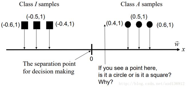
分割点为:
因此,值大于此分割点时属于Class A,反之则属于Class I

算法分析
由于是两类数据,因此我们只需要将数据投影到一条直线上即可。假设我们的投影直线是向量 w ,则对任意一个样本本 xi ,它在直线w的投影为 wTxi ,对于我们的两个类别的中心点 μ0,μ1 ,在在直线w的投影为 wTμ0 和 wTμ1 。由于LDA需要让不同类别的数据的类别中心之间的距离尽可能的大,也就是我们要最大化 ||wTμ0−wTμ1||22 ,同时我们希望同一种类别数据的投影点尽可能的接近,也就是要同类样本投影点的协方差 wTΣ0w 和 wTΣ1w 尽可能的小,即最小化 wTΣ0w+wTΣ1w 。
代入上面的 类内散度矩阵Sw与类间散度矩阵Sb 可以得出
利用广义瑞利商的性质,我们知道我们的J(w)最大值为矩阵 S−1wSb 的最大特征值,而对应的w为 S−1wSb 的最大特征值对应的特征向量。
注意到对于二类的时候, Sbw 的方向恒为 μ0−μ1 ,不妨令 Sbw=λ(μ0−μ1) 将其带入 (S−1wSb)w=λw 可以得出 w=S−1w(μ0−μ1)
示例代码
myfld.m
% FLD classifies an input sample into either class 1 or class 2.
%
%   [output_class w] = myfld(input_sample, class1_samples, class2_samples)
%   classifies an input sample into either class 1 or class 2,
%   from samples of class 1 (class1_samples) and samples of
%   class 2 (class2_samples).
%
% Input parameters:
% input_sample = an input sample
%   - The number of dimensions of the input sample is N.
%
% class1_samples = a NC1xN matrix
%   - class1_samples contains all samples taken from class 1.
%   - The number of samples is NC1.
%   - The number of dimensions of each sample is N.
%
% class2_samples = a NC2xN matrix
%   - class2_samples contains all samples taken from class 2.
%   - The number of samples is NC2.
%   - NC1 and NC2 do not need to be the same.
%   - The number of dimensions of each sample is N.
%
% Output parameters:
% output_class = the class to which input_sample belongs.
%   - output_class should have the value either 1 or 2.
%
% w = weight vector.
%   - The vector length must be one.
%
function [output_class w] = myfld(input_sample, class1_samples, class2_samples)
[m1, n1] = size(class1_samples);
[m2, n2] = size(class2_samples);
mu1 = sum(class1_samples) / size(class1_samples, 1);
mu2 = sum(class2_samples) / size(class2_samples, 1);
s1 = 0;
s2 = 0;

for i = 1:m1
    s1 = s1 + (class1_samples(i,:) - mu1)' * (class1_samples(i,:) - mu1);
end
for i = 1:m2
    s2 = s2 + (class2_samples(i,:) - mu2)' * (class2_samples(i,:) - mu2);
end
sw = s1 + s2;
w = inv(sw)' * (mu1 - mu2)';
w1 = w(1) / (w(1) * w(1) + w(2) * w(2))^0.5;
w2 = w(2) / (w(1) * w(1) + w(2) * w(2))^0.5;
w = [w1; w2];
separationPoint = (mu1 + mu2) * w * 0.5;
output_class = (input_sample * w < separationPoint) + 1;
总结
对比PCA
LDA用于降维,和PCA有很多相同,也有很多不同的地方,因此值得好好的比较一下两者的降维异同点。
相同点:
- 两者均可以对数据进行降维。
- 两者在降维时均使用了矩阵特征分解的思想。
- 两者都假设数据符合高斯分布。
不同点:
- LDA是有监督的降维方法,而PCA是无监督的降维方法
- LDA降维最多降到类别数k-1的维数,而PCA没有这个限制。
- LDA除了可以用于降维,还可以用于分类。
- LDA选择分类性能最好的投影方向,而PCA选择样本点投影具有最大方差的方向。
这点可以从下图形象的看出,在某些数据分布下LDA比PCA降维较优。


LDA cons and pros
主要优点:
- 在降维过程中可以使用类别的先验知识经验,而像PCA这样的无监督学习则无法使用类别先验知识。
- LDA在样本分类信息依赖均值而不是方差的时候,比PCA之类的算法较优。
主要缺点:
- LDA不适合对非高斯分布样本进行降维,PCA也有这个问题。
- LDA降维最多降到类别数k-1的维数,如果我们降维的维度大于k-1,则不能使用LDA。(当然目前有一些LDA的进化版算法可以绕过这个问题)
- LDA在样本分类信息依赖方差而不是均值的时候,降维效果不好。
- LDA可能过度拟合数据。
参考文献
- http://blog.csdn.net/warmyellow/article/details/5454943
- http://www.cnblogs.com/pinard/p/6244265.html
- http://en.wikipedia.org/wiki/Linear_discriminant_analysis