- 深度学习框架 人工智能操作系统 训练&前向推理 PyTorch Tensorflow MindSpore caffe 张量加速引擎TBE 深度学习编译器 多面体 polyhedral AI集群框架
EwenWanW
深度学习人工智能pytorch深度学习编译器
深度学习框架人工智能操作系统训练&前向推理深度学习框架发展到今天,目前在架构上大体已经基本上成熟并且逐渐趋同。无论是国外的Tensorflow、PyTorch,亦或是国内最近开源的MegEngine、MindSpore,目前基本上都是支持EagerMode和GraphMode两种模式。AI嵌入式框架OneFlow&清华计图Jittor&华为深度学习框架MindSpore&旷视深度学习框架MegEn
- Caffeine 与 Guava Cache
雨季里的向日葵
java
一、概要1.1背景在项目开发中,为提升系统性能,减少IO开销,本地缓存是必不可少的。最常见的本地缓存是Guava和Caffeine,Caffeine是基于GoogleGuavaCache设计经验改进的结果,相较于Guava在性能和命中率上更具有效率。1.2应用场景愿意消耗一些内存空间来提升速度预料到某些键会被多次查询缓存中存放的数据总量不会超出内存容量二、GuavaCache2.1GuavaCac
- OSError: [WinError 126] 找不到指定的模块---caffe2_detectron_ops_gpu.dll
努力的小柚
python运行问题pythonpytorch
代码复现记录:问题:OSError:[WinError126]找不到指定的模块。Errorloading"C:\Anaconda\Anaconda3\envs\TIN\lib\site-packages\torch\lib\caffe2_detectron_ops_gpu.dll"oroneofitsdependencies.在搜索很多关于无法查找到caffe2_detectron_ops_gpu
- caffe/PyTorch/TensorFlow 在Jupyter Notebook GPU中运用
俊俏的萌妹纸
caffe人工智能深度学习
在JupyterNotebook中使用Caffe框架并利用GPU加速,可以实现多种效果和目的,主要集中在深度学习领域。以下是一些主要的应用场景:快速训练模型:GPU加速可以显著提高模型训练的速度。对于大型数据集和复杂的神经网络结构,使用GPU可以大大减少训练时间。实时数据增强:在训练过程中,可以实时地对输入数据进行变换和增强,以提高模型的泛化能力。GPU加速使得这些操作更加高效。大规模数据处理:深
- Linux下Caffe、Docker、Tensorflow、PyTorch环境搭建(CentOS 7)
SnailTyan
文章作者:Tyan博客:noahsnail.com|CSDN|注:模型的训练、测试、部署都可以通过Docker环境完成,环境问题会更少。1.CUDA8.0安装CUDA8.0Configenvvariables#CUDAPATHexportPATH="/usr/local/cuda-8.0/bin:$PATH"#CUDALDLIBRARY_PATHexportLD_LIBRARY_PATH="/us
- JVM级缓存本地缓存Caffeine
旺仔爱Java
JVM专题jvmJVM缓存本地缓存CaffeineGuavaCache
JVM级缓存本地缓存Caffeine和GuavaCache前言一、创建缓存的代码逻辑二、Caffeine的优化方面淘汰算法W-TinyLFU三、Caffeine的业务使用总结前言最新的Java面试题,技术栈涉及Java基础、集合、多线程、Mysql、分布式、Spring全家桶、MyBatis、Dubbo、缓存、消息队列、Linux…等等,会持续更新。一、创建缓存的代码逻辑Caffeine:publ
- 面试redis篇-04缓存雪崩
卡搜偶
缓存面试redis
原理缓存雪崩:是指在同一时段大量的缓存key同时失效或者Redis服务宕机,导致大量请求到达数据库,带来巨大压力。解决方案:给不同的Key的TTL添加随机值利用Redis集群提高服务的可用性(哨兵模式、集群模式)给缓存业务添加降级限流策略(ngxin或springcloudgateway)给业务添加多级缓存(Guava或Caffeine)问答面试官:什么是缓存雪崩?怎么解决?回答:缓存雪崩意思是设
- 深度学习主流开源框架:Caffe、TensorFlow、Pytorch、Theano、Keras、MXNet、Chainer
seasonsyy
深度学习小知识深度学习开源框架pytorch
2.6深度学习主流开源框架表2.1深度学习主流框架参数对比框架关键词总结框架关键词基本数据结构(都是高维数组)Caffe“在工业中应用较为广泛”,“编译安装麻烦一点”BlobTensorFlow“安装简单pip”TensorPytorch“定位:快速实验研究”,“简单”,“灵活”TensorTheanoד用于处理大规模神经网络的训练”,“不支持移动设备”,“不能应用于工业环境”,“编译复杂模型时
- MMsegmentation-随机初始化
SatVision炼金士
mmalb-炼金术python
系列文章目录文章目录系列文章目录前言一、初始化单个模块二、初始化多个模块总结前言mmlab下游分支调用权重随机初始化使用参考mmengine的说明文档mmengine支持模型初始化方法包括:BaseInit,Caffe2XavierInit,ConstantInit,KaimingInit,NormalInit,PretrainedInit,TruncNormalInit,UniformInit,
- 解决:源码安装caffe时遇到libcudnn.so: file not recognized问题
Gracie丹妮
参考教程(19条消息)ubuntu16.04下Detectron+caffe2(Pytorch)安装配置过程_张家坎的博客-CSDN博客_caffe2_detectron_ops_gpu.dllhttps://blog.csdn.net/u014236392/article/details/81117287安装caffe2执行sudomakeinstall之后遇到如下问题:/home/Xdn/cu
- 进场 行礼 问候 退场
东方芭蕾Lily
1.当听到响铃声,按编号排队依次进入考场。tips:面带微笑,优雅自信且有礼貌的边看着考试官边跑到准备问好的位置。步伐轻盈像一阵风样,到位置站好一位脚,保持挺拔向上体态。小仙女就是你们。2.行礼问候Examier:(考试官)GillianMccafferyGoodmorning/afternoongirlsGoodmorning/afrernoonmadamorMs.MccafferyQuesti
- YOLOv5独家改进:上采样算子 | 超轻量高效动态上采样DySample,效果秒杀CAFFE,助力小目标检测
AI小怪兽
YOLOv5原创自研YOLOcaffe目标检测深度学习人工智能
本文独家改进:一种超轻量高效动态上采样DySample,具有更少的参数、FLOPs,效果秒杀CAFFE和YOLOv5网络中的nn.Upsample在多个数据集下验证能够涨点,尤其在小目标检测领域涨点显著。收录YOLOv5原创自研https://blog.csdn.net/m0_63774211/category_12511931.html全网独家首发创新(原创),适合paper!!!2024年计算
- caffez转ncnn,及环境配置
宁静深远
软件安装
一、安装ncnn1、安装protobuf(a)、gitclonehttps://github.com/google/protobuf(b)、自动生成configure配置文件,运行:./autogen.sh(c)、配置环境:./configure(d)、编译源代码:make(e)、安装:sudomakeinstall(f)、刷新动态库:sudoldconfig2、安装ncnn(a)、mkdirco
- 最新姿态估计研究进展
a微风掠过
最新姿态估计研究进展自上而下:就是先检测包含人的框,即humanproposal,然后对框子中的人进行姿态估计。一般RCNN(区域CNN就是这个思路)自下而上:先检测keypoint,然后根据热力图、点与点之间连接的概率,根据图论知识,基于PAF(部分亲和字段)将关键点连接起来,将关键点分组到人。1、CMU:openpose研究多人的姿态估计运行环境:caffe自下而上,关键点被分组到人的实例时间
- 智慧云智能教育考试平台展示
barry200890
springbootvue考试javavue.js小程序
智慧云智能教育平台项目简介技术架构1.1后端技术栈:*基于SpringBoot+MybatisPlus+Shiro+mysql5.7+redis+websocket构建.*使用jdk1.8的新特性如:caffeine缓存,lambda表达式.1.2前端技术:*Vue*Vuex*Vxe-Table(文档地址:https://gitee.com/xuliangzhan_admin/vxe-table)
- what is SSD|Single Shot MultiBox Detector
Woooooooooooooo
文章摘选自多篇文章,仅用于学习,在此表示感谢,若有侵权请联系,感谢论文下载地址:https://arxiv.org/abs/1512.02325论文代码:https://github.com/weiliu89/caffe/tree/ssd省去了区域建议网络,直接使用不同尺度featuremap中的cell得到priodbox(和anchor类似),利用卷积可以直接得到box的回归和score而不需
- caffe中的参考模型
雨住多一横
RCNNmode_reference_rcnn_ilsvrc13l.pngcaffenet用于Flickrstyle数据集model_finetune_flickr_style.pngAlexNetmodel_alexnet.pnggooglenetmodel_googlenet.pngcaffenetmodel_reference_caffenet.png
- RT-DETR算法优化改进:上采样算子 | 超轻量高效动态上采样DySample,效果秒杀CAFFE,助力小目标检测
AI小怪兽
RT-DETR魔术师算法caffe目标检测YOLO深度学习人工智能
本文独家改进:一种超轻量高效动态上采样DySample,具有更少的参数、FLOPs,效果秒杀CAFFE和YOLOv8网络中的nn.Upsample在多个数据集下验证能够涨点,尤其在小目标检测领域涨点显著。RT-DETR魔术师专栏介绍:https://blog.csdn.net/m0_63774211/category_12497375.html✨✨✨魔改创新RT-DETR引入前沿顶会创新(CVPR
- 「性能提升」扩展 Spring Cache 支持多级缓存
冷冷zz
为什么多级缓存缓存的引入是现在大部分系统所必须考虑的redis作为常用中间件,虽然我们一般业务系统(毕竟业务量有限)不会遇到如下图在随着data-size的增大和数据结构的复杂的造成性能下降,但网络IO消耗会成为整个调用链路中不可忽视的部分。尤其在微服务架构中,一次调用往往会涉及多次调用例如pigoauth2.0的client认证Caffeine来自未来的本地内存缓存,性能比如常见的内存缓存实现性
- Spring Cache
duration~
spring-bootspringjava后端
目录标题SpringCache1介绍2常用注解3入门SpringCache1介绍SpringCache是一个框架,实现了基于注解的缓存功能,只需要简单地加一个注解,就能实现缓存功能。SpringCache提供了一层抽象,底层可以切换不同的缓存实现,例如:EHCacheCaffeineRedis(常用)起步依赖:org.springframework.bootspring-boot-starter-
- Caffeine与Spring cache的各种注解操作
500了
springjava后端
前言Caffeine是一个基于Java8的进程内缓存框架,它使用乐观锁技术来提高并发吞吐量,并被誉为最快的缓存之一。Caffeine是内存型缓存,即缓存与调用者属于同一个应用,具体地说是属于同一个JVM。它的设计目标是提供高性能、高命中率以及低内存占用的本地缓存解决方案,被描述为GuavaCache的加强版和“新一代缓存”。关于Caffeine的使用,其提供了多种灵活的配置选项:自动加载数据:可以
- 缓存组件Caffeine的使用
月月大王
Java#工具类缓存
caffeine是一个高性能的缓存组件,在需要缓存数据,但数据量不算太大,不想引入redis的时候,caffeine就是一个不错的选择。可以把caffeine理解为一个简单的redis。1、导入依赖com.github.ben-manes.caffeinecaffeine2.9.3导入是要注意版本,最开始我用的版本是3.1.1,不过启动是的时候会报错,这是因为我用的是jdk1.8,需要降低一下版本
- Makefile.config
walkMAN_aholic
##Refertohttp://caffe.berkeleyvision.org/installation.html#Contributionssimplifyingandimprovingourbuildsystemarewelcome!#cuDNNaccelerationswitch(uncommenttobuildwithcuDNN).USE_CUDNN:=1#CPU-onlyswitch(
- 缓存Caffeine之W-TinyLFU淘汰策略
georgesnoopy
guava缓存java淘汰策略Caffeine
我们常见的缓存是基于内存的缓存,但是单机的内存是有限的,不能让缓存数据撑爆内存,所有需要缓存淘汰机制。https://mp.csdn.net/editor/html/115872837中大概说明了LRU的缓存淘汰机制,以及基于LRU的著名实现guavacache。除了LRU淘汰策略外,其是常见的还有FIFO以及LFU,只是说目前用的最多的是LRU。LRULRU记录了缓存中数据项的访问时间,在缓存数
- Caffeine史上最快的内存缓存
奇遇少年
缓存java
引言在现代的Web应用程序中,缓存是提升性能,减少数据库负载,加快响应速度的关键技术之一。SpringBoot作为一个简化Spring应用开发的框架,提供了与多种缓存技术集成的支持。Caffeine是一个高性能,灵活的缓存库,它可以作为本地缓存在Java应用中广泛使用。本文将详细介绍如何在SpringBoot项目中集成Caffeine缓存,并通过一个实例来展示它的使用。什么是Caffeine缓存?
- 如何解决caffe和video-caffe不能使用cudnn8编译的问题
Arnold-FY-Chen
video-caffe深度学习Caffevideo-caffecaffe深度学习cudnn8cudnn
因为caffe之类的代码很久不更新了,只支持到了使用cudnn7.x,在使用了cudnn8的环境下编译caffe或video-caffe时,会在src/caffe/layers/cudnn_conv_layer.cpp等文件里出错:error:identifier"CUDNN_CONVOLUTION_FWD_SPECIFY_WORKSPACE_LIMIT"isundefinederror:iden
- Redis 6.0 客户端缓存
极简博客
javaredis
不难发现,我们经常将Redis作为系统的缓存服务,但你有没有发现。在我们每次操作Redis时,都需要发送网络请求。这样就避免不了网络的开销。但如何解决这个问题呢?我们引入了本地缓存来解决此问题。查询逻辑从先前的直接查询转变为:先通过查询本地缓存,不存在再去远程查找然后设置到本地缓存-适用于分布式客户端缓存。有没有感觉像我们使用过的本地缓存Guava、Caffeine等一样?有啥特别的?这里Redi
- [图像算法]-(yolov5.train)-GPU架构中的半精度fp16与单精度fp32计算
蒸饺与白茶
GPU架构中的半精度与单精度计算 由于项目原因,我们需要对darknet中卷积层进行优化,然而对于像caffe或者darknet这类深度学习框架来说,都已经将卷积运算转换成了矩阵乘法,从而可以方便调用cublas库函数和cudnn里tiling过的矩阵乘。 CUDA在推出7.5的时候提出了可以计算16位浮点数据的新特性。定义了两种新的数据类型half和half2.之前有师弟已经DEMO过半精度
- caffe搭建深度神经网络
A异乡人_7a44
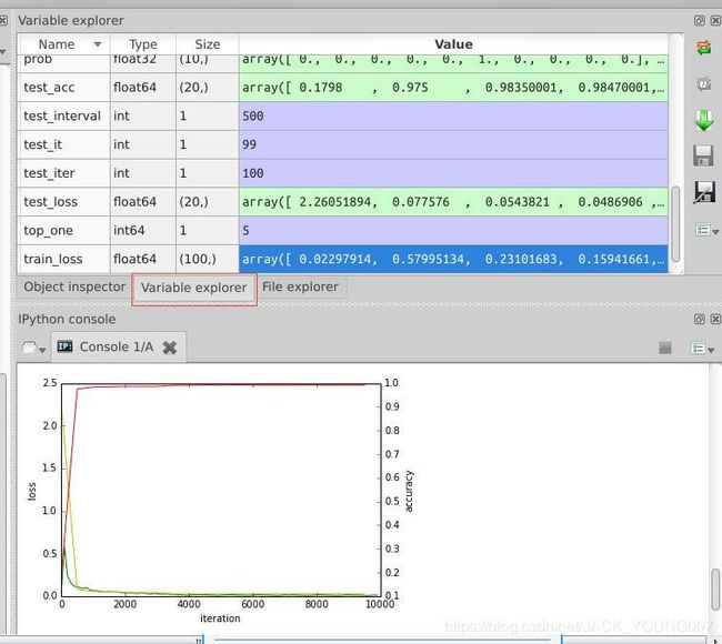
利用Caffe进行深度神经网络训练第一步需要搞懂几个重要文件:solver.prototxttrain_val.prototxttrain.shsolver.prototxtsolver这个文件主要存放模型训练所用到的一些超参数:net:=指定待训练模型结构文件,即train_val.prototxttest_interval:=测试间隔,即每隔多少次迭代进行一次测试test_initializa
- deep-visualization-toolbox可视化安装
2014wzy
caffe框架
运行环境:Linux+caffe步骤:Step0:Compilemasterbranchofcaffe本代码运行的前提是,配置过caffe。因为配置caffe的过程中会出现一些依赖库,正是本代码所需要的。http://blog.csdn.NET/u011204487/article/details/51596471是配置caffe的过程。注意Makefile.config中的CPU_ONLY:=1
- ios内付费
374016526
ios内付费
近年来写了很多IOS的程序,内付费也用到不少,使用IOS的内付费实现起来比较麻烦,这里我写了一个简单的内付费包,希望对大家有帮助。
具体使用如下:
这里的sender其实就是调用者,这里主要是为了回调使用。
[KuroStoreApi kuroStoreProductId:@"产品ID" storeSender:self storeFinishCallBa
- 20 款优秀的 Linux 终端仿真器
brotherlamp
linuxlinux视频linux资料linux自学linux教程
终端仿真器是一款用其它显示架构重现可视终端的计算机程序。换句话说就是终端仿真器能使哑终端看似像一台连接上了服务器的客户机。终端仿真器允许最终用户用文本用户界面和命令行来访问控制台和应用程序。(LCTT 译注:终端仿真器原意指对大型机-哑终端方式的模拟,不过在当今的 Linux 环境中,常指通过远程或本地方式连接的伪终端,俗称“终端”。)
你能从开源世界中找到大量的终端仿真器,它们
- Solr Deep Paging(solr 深分页)
eksliang
solr深分页solr分页性能问题
转载请出自出处:http://eksliang.iteye.com/blog/2148370
作者:eksliang(ickes) blg:http://eksliang.iteye.com/ 概述
长期以来,我们一直有一个深分页问题。如果直接跳到很靠后的页数,查询速度会比较慢。这是因为Solr的需要为查询从开始遍历所有数据。直到Solr的4.7这个问题一直没有一个很好的解决方案。直到solr
- 数据库面试题
18289753290
面试题 数据库
1.union ,union all
网络搜索出的最佳答案:
union和union all的区别是,union会自动压缩多个结果集合中的重复结果,而union all则将所有的结果全部显示出来,不管是不是重复。
Union:对两个结果集进行并集操作,不包括重复行,同时进行默认规则的排序;
Union All:对两个结果集进行并集操作,包括重复行,不进行排序;
2.索引有哪些分类?作用是
- Android TV屏幕适配
酷的飞上天空
android
先说下现在市面上TV分辨率的大概情况
两种分辨率为主
1.720标清,分辨率为1280x720.
屏幕尺寸以32寸为主,部分电视为42寸
2.1080p全高清,分辨率为1920x1080
屏幕尺寸以42寸为主,此分辨率电视屏幕从32寸到50寸都有
适配遇到问题,已1080p尺寸为例:
分辨率固定不变,屏幕尺寸变化较大。
如:效果图尺寸为1920x1080,如果使用d
- Timer定时器与ActionListener联合应用
永夜-极光
java
功能:在控制台每秒输出一次
代码:
package Main;
import javax.swing.Timer;
import java.awt.event.*;
public class T {
private static int count = 0;
public static void main(String[] args){
- Ubuntu14.04系统Tab键不能自动补全问题解决
随便小屋
Ubuntu 14.04
Unbuntu 14.4安装之后就在终端中使用Tab键不能自动补全,解决办法如下:
1、利用vi编辑器打开/etc/bash.bashrc文件(需要root权限)
sudo vi /etc/bash.bashrc
接下来会提示输入密码
2、找到文件中的下列代码
#enable bash completion in interactive shells
#if
- 学会人际关系三招 轻松走职场
aijuans
职场
要想成功,仅有专业能力是不够的,处理好与老板、同事及下属的人际关系也是门大学问。如何才能在职场如鱼得水、游刃有余呢?在此,教您简单实用的三个窍门。
第一,多汇报
最近,管理学又提出了一个新名词“追随力”。它告诉我们,做下属最关键的就是要多请示汇报,让上司随时了解你的工作进度,有了新想法也要及时建议。不知不觉,你就有了“追随力”,上司会越来越了解和信任你。
第二,勤沟通
团队的力
- 《O2O:移动互联网时代的商业革命》读书笔记
aoyouzi
读书笔记
移动互联网的未来:碎片化内容+碎片化渠道=各式精准、互动的新型社会化营销。
O2O:Online to OffLine 线上线下活动
O2O就是在移动互联网时代,生活消费领域通过线上和线下互动的一种新型商业模式。
手机二维码本质:O2O商务行为从线下现实世界到线上虚拟世界的入口。
线上虚拟世界创造的本意是打破信息鸿沟,让不同地域、不同需求的人
- js实现图片随鼠标滚动的效果
百合不是茶
JavaScript滚动属性的获取图片滚动属性获取页面加载
1,获取样式属性值
top 与顶部的距离
left 与左边的距离
right 与右边的距离
bottom 与下边的距离
zIndex 层叠层次
例子:获取左边的宽度,当css写在body标签中时
<div id="adver" style="position:absolute;top:50px;left:1000p
- ajax同步异步参数async
bijian1013
jqueryAjaxasync
开发项目开发过程中,需要将ajax的返回值赋到全局变量中,然后在该页面其他地方引用,因为ajax异步的原因一直无法成功,需将async:false,使其变成同步的。
格式:
$.ajax({ type: 'POST', ur
- Webx3框架(1)
Bill_chen
eclipsespringmaven框架ibatis
Webx是淘宝开发的一套Web开发框架,Webx3是其第三个升级版本;采用Eclipse的开发环境,现在支持java开发;
采用turbine原型的MVC框架,扩展了Spring容器,利用Maven进行项目的构建管理,灵活的ibatis持久层支持,总的来说,还是一套很不错的Web框架。
Webx3遵循turbine风格,velocity的模板被分为layout/screen/control三部
- 【MongoDB学习笔记五】MongoDB概述
bit1129
mongodb
MongoDB是面向文档的NoSQL数据库,尽量业界还对MongoDB存在一些质疑的声音,比如性能尤其是查询性能、数据一致性的支持没有想象的那么好,但是MongoDB用户群确实已经够多。MongoDB的亮点不在于它的性能,而是它处理非结构化数据的能力以及内置对分布式的支持(复制、分片达到的高可用、高可伸缩),同时它提供的近似于SQL的查询能力,也是在做NoSQL技术选型时,考虑的一个重要因素。Mo
- spring/hibernate/struts2常见异常总结
白糖_
Hibernate
Spring
①ClassNotFoundException: org.aspectj.weaver.reflect.ReflectionWorld$ReflectionWorldException
缺少aspectjweaver.jar,该jar包常用于spring aop中
②java.lang.ClassNotFoundException: org.sprin
- jquery easyui表单重置(reset)扩展思路
bozch
formjquery easyuireset
在jquery easyui表单中 尚未提供表单重置的功能,这就需要自己对其进行扩展。
扩展的时候要考虑的控件有:
combo,combobox,combogrid,combotree,datebox,datetimebox
需要对其添加reset方法,reset方法就是把初始化的值赋值给当前的组件,这就需要在组件的初始化时将值保存下来。
在所有的reset方法添加完毕之后,就需要对fo
- 编程之美-烙饼排序
bylijinnan
编程之美
package beautyOfCoding;
import java.util.Arrays;
/*
*《编程之美》的思路是:搜索+剪枝。有点像是写下棋程序:当前情况下,把所有可能的下一步都做一遍;在这每一遍操作里面,计算出如果按这一步走的话,能不能赢(得出最优结果)。
*《编程之美》上代码有很多错误,且每个变量的含义令人费解。因此我按我的理解写了以下代码:
*/
- Struts1.X 源码分析之ActionForm赋值原理
chenbowen00
struts
struts1在处理请求参数之前,首先会根据配置文件action节点的name属性创建对应的ActionForm。如果配置了name属性,却找不到对应的ActionForm类也不会报错,只是不会处理本次请求的请求参数。
如果找到了对应的ActionForm类,则先判断是否已经存在ActionForm的实例,如果不存在则创建实例,并将其存放在对应的作用域中。作用域由配置文件action节点的s
- [空天防御与经济]在获得充足的外部资源之前,太空投资需有限度
comsci
资源
这里有一个常识性的问题:
地球的资源,人类的资金是有限的,而太空是无限的.....
就算全人类联合起来,要在太空中修建大型空间站,也不一定能够成功,因为资源和资金,技术有客观的限制....
&
- ORACLE临时表—ON COMMIT PRESERVE ROWS
daizj
oracle临时表
ORACLE临时表 转
临时表:像普通表一样,有结构,但是对数据的管理上不一样,临时表存储事务或会话的中间结果集,临时表中保存的数据只对当前
会话可见,所有会话都看不到其他会话的数据,即使其他会话提交了,也看不到。临时表不存在并发行为,因为他们对于当前会话都是独立的。
创建临时表时,ORACLE只创建了表的结构(在数据字典中定义),并没有初始化内存空间,当某一会话使用临时表时,ORALCE会
- 基于Nginx XSendfile+SpringMVC进行文件下载
denger
应用服务器Webnginx网络应用lighttpd
在平常我们实现文件下载通常是通过普通 read-write方式,如下代码所示。
@RequestMapping("/courseware/{id}")
public void download(@PathVariable("id") String courseID, HttpServletResp
- scanf接受char类型的字符
dcj3sjt126com
c
/*
2013年3月11日22:35:54
目的:学习char只接受一个字符
*/
# include <stdio.h>
int main(void)
{
int i;
char ch;
scanf("%d", &i);
printf("i = %d\n", i);
scanf("%
- 学编程的价值
dcj3sjt126com
编程
发一个人会编程, 想想以后可以教儿女, 是多么美好的事啊, 不管儿女将来从事什么样的职业, 教一教, 对他思维的开拓大有帮助
像这位朋友学习:
http://blog.sina.com.cn/s/articlelist_2584320772_0_1.html
VirtualGS教程 (By @林泰前): 几十年的老程序员,资深的
- 二维数组(矩阵)对角线输出
飞天奔月
二维数组
今天在BBS里面看到这样的面试题目,
1,二维数组(N*N),沿对角线方向,从右上角打印到左下角如N=4: 4*4二维数组
{ 1 2 3 4 }
{ 5 6 7 8 }
{ 9 10 11 12 }
{13 14 15 16 }
打印顺序
4
3 8
2 7 12
1 6 11 16
5 10 15
9 14
13
要
- Ehcache(08)——可阻塞的Cache——BlockingCache
234390216
并发ehcacheBlockingCache阻塞
可阻塞的Cache—BlockingCache
在上一节我们提到了显示使用Ehcache锁的问题,其实我们还可以隐式的来使用Ehcache的锁,那就是通过BlockingCache。BlockingCache是Ehcache的一个封装类,可以让我们对Ehcache进行并发操作。其内部的锁机制是使用的net.
- mysqldiff对数据库间进行差异比较
jackyrong
mysqld
mysqldiff该工具是官方mysql-utilities工具集的一个脚本,可以用来对比不同数据库之间的表结构,或者同个数据库间的表结构
如果在windows下,直接下载mysql-utilities安装就可以了,然后运行后,会跑到命令行下:
1) 基本用法
mysqldiff --server1=admin:12345
- spring data jpa 方法中可用的关键字
lawrence.li
javaspring
spring data jpa 支持以方法名进行查询/删除/统计。
查询的关键字为find
删除的关键字为delete/remove (>=1.7.x)
统计的关键字为count (>=1.7.x)
修改需要使用@Modifying注解
@Modifying
@Query("update User u set u.firstna
- Spring的ModelAndView类
nicegege
spring
项目中controller的方法跳转的到ModelAndView类,一直很好奇spring怎么实现的?
/*
* Copyright 2002-2010 the original author or authors.
*
* Licensed under the Apache License, Version 2.0 (the "License");
* yo
- 搭建 CentOS 6 服务器(13) - rsync、Amanda
rensanning
centos
(一)rsync
Server端
# yum install rsync
# vi /etc/xinetd.d/rsync
service rsync
{
disable = no
flags = IPv6
socket_type = stream
wait
- Learn Nodejs 02
toknowme
nodejs
(1)npm是什么
npm is the package manager for node
官方网站:https://www.npmjs.com/
npm上有很多优秀的nodejs包,来解决常见的一些问题,比如用node-mysql,就可以方便通过nodejs链接到mysql,进行数据库的操作
在开发过程往往会需要用到其他的包,使用npm就可以下载这些包来供程序调用
&nb
- Spring MVC 拦截器
xp9802
spring mvc
Controller层的拦截器继承于HandlerInterceptorAdapter
HandlerInterceptorAdapter.java 1 public abstract class HandlerInterceptorAdapter implements HandlerIntercep