10_Introduction to Artificial Neural Networks w Keras_5

10_Introduction to Artificial Neural Networks with Keras_HuberLoss_astype_dtype_DNN_MLP_G.gv.pdf_mnist
https://blog.csdn.net/Linli522362242/article/details/106433059

10_Introduction to Artificial Neural Networks with Keras_2_tensorflow2.1_Anaconda3-2019.10(python3.7.4)
https://blog.csdn.net/Linli522362242/article/details/106537459

10_Introduction to Artificial Neural Networks w Keras_3_FashionMNIST_pydot_sparse_shift(0.)_plt_imgs
https://blog.csdn.net/Linli522362242/article/details/106562190

10_Introduction to Artificial Neural_4_Regression MLP_Sequential_Subclassing_saveMode_Callback_board
https://blog.csdn.net/Linli522362242/article/details/106582512

10_5_IMDB_newswires_house prices_Self-supervised_Hold-out_K-fold_L2_dropout_overfit_TP_metrics
https://blog.csdn.net/Linli522362242/article/details/106755312

import tensorflow as tf
from tensorflow import keras
from sklearn.datasets import fetch_california_housing
from sklearn.model_selection import train_test_split
from sklearn.preprocessing import StandardScaler

housing = fetch_california_housing()

X_train_full, X_test, y_train_full, y_test = train_test_split( housing.data, housing.target, 
                                                              random_state=42)
X_train, X_valid, y_train, y_valid = train_test_split( X_train_full, y_train_full, 
                                                      random_state=42)

scaler = StandardScaler()
X_train = scaler.fit_transform(X_train)
X_valid = scaler.transform(X_valid)
X_test = scaler.transform(X_test)

X_train_A, X_train_B = X_train[:, :5], X_train[:, 2:]
X_valid_A, X_valid_B = X_valid[:, :5], X_valid[:, 2:]
X_test_A, X_test_B = X_test[:, :5], X_test[:, 2:]

X_new_A, X_new_B = X_test_A[:3], X_test_B[:3]

Fine-Tuning Neural Network Hyperparameters

     The flexibility of neural networks is also one of their main drawbacks: there are many hyperparameters to tweak. Not only can you use any imaginable network architecture, but even in a simple MLP you can change the number of layers, the number of neurons per layer, the type of activation function to use in each layer, the weight initialization logic, and much more. How do you know what combination of hyperparameters is the best for your task?

     One option is to simply try many combinations of hyperparameters and see which one works best on the validation set (or use K-fold cross-validation). For example, we can use GridSearchCV or RandomizedSearchCV to explore the hyperparameter space, as we did in Cp2( https://blog.csdn.net/Linli522362242/article/details/103587172). To do this, we need to wrap our Keras models in objects that mimic[ˈmɪmɪk]模仿 regular Scikit-Learn regressors. The first step is to create a function that will build and compile a Keras model, given a set of hyperparameters:

Hyperparameter Tuning

from tensorflow import keras
import numpy as np
import tensorflow as tf

keras.backend.clear_session()
np.random.seed(42)
tf.random.set_seed(42)

def build_model( n_hidden=1, n_neurons=30, learning_rate=3e-3, input_shape=[8] ):
    model = keras.models.Sequential()
    model.add( keras.layers.InputLayer( input_shape=input_shape ) ) #input layer
    for layer in range(n_hidden):
        model.add( keras.layers.Dense(n_neurons, activation='relu') )#hidden layers
    model.add(keras.layers.Dense(1)) #output layer
    optimizer = keras.optimizers.SGD( lr=learning_rate )
    model.compile(loss="mse", optimizer=optimizer)
    return model

      This function creates a simple Sequential model for univariate[junɪ'veərɪrt]单变量 regression (only one output neuron), with the given input shape and the given number of hidden layers and neurons, and it compiles it using an SGD optimizer configured with the specified learning rate. It is good practice to provide reasonable defaults to as many hyperparameters as you can, as Scikit-Learn does.

Next, let’s create a KerasRegressor based on this build_model() function:

keras_reg = keras.wrappers.scikit_learn.KerasRegressor( build_model )

     The KerasRegressor object is a thin wrapper around the Keras model built using build_model(). Since we did not specify any hyperparameters when creating it, it will use the default hyperparameters we defined in build_model(). Now we can use
this object like a regular Scikit-Learn regressor: we can train it using its fit() method, then evaluate it using its score() method, and use it to make predictions using its predict() method, as you can see in the following code:

keras_reg.fit( X_train, y_train, epochs=100, validation_data=(X_valid, y_valid), 
              callbacks=[ keras.callbacks.EarlyStopping(patience=10) ]
             )

 

... ...

mse_test = keras_reg.score(X_test, y_test) #Returns the mean loss(mse) on the given test data and labels.

 

mse_test

 

X_new= X_test[:3]
y_pred = keras_reg.predict(X_new)
y_pred

 
     Note that any extra parameter you pass to the fit() method will get passed to the underlying Keras model. Also note that the score will be the opposite of the MSE because Scikit-Learn wants scores, not losses (i.e., higher should be better).
https://blog.csdn.net/Linli522362242/article/details/103587172

     We don’t want to train and evaluate a single model like this, though we want to train hundreds of variants and see which one performs best on the validation set. Since there are many hyperparameters, it is preferable to use a randomized search rather than grid search (as we discussed in Cp2 https://blog.csdn.net/Linli522362242/article/details/103646927). Let’s try to explore the number of hidden layers, the number of neurons, and the learning rate:

np.random.seed(42)
tf.random.set_seed(42)

from scipy.stats import reciprocal
from sklearn.model_selection import RandomizedSearchCV

param_distribs = {
    "n_hidden" : [0,1,2,3],
    "n_neurons" : np.arange(1,100),
    "learning_rate" : reciprocal(3e-4, 3e-2) #  https://blog.csdn.net/Linli522362242/article/details/103646927
}                 # reciprocal distribution, log(this distribution) is a uniform distribution within a given range
#The reciprocal distribution is useful when you have no idea what the scale范围大小 of the hyperparameter should be
rnd_search_cv = RandomizedSearchCV( keras_reg, param_distribs, n_iter=10, cv=3, verbose=2 )
rnd_search_cv.fit( X_train, y_train, epochs=100, validation_data = (X_valid, y_valid),
                   callbacks = [keras.callbacks.EarlyStopping(patience=10)]#base on val_loss
                 )

 

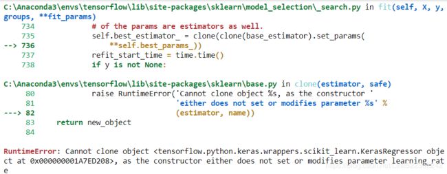
Warning: the following cell crashes at the end of training. This seems to be caused by Keras issue #13586, which was triggered by a recent change in Scikit-Learn. Pull Request #13598 seems to fix the issue, so this problem should be resolved soon. 

 
... ...

RuntimeError: Cannot clone object , as the constructor either does not set or modifies parameter learning_rate

RuntimeError: Cannot clone object , as the constructor either does not set or modifies parameter learning_rate

rnd_search_cv.best_params_

 {'learning_rate': 0.0033625641252688094, 'n_hidden': 2, 'n_neurons': 42}

rnd_search_cv.best_score_

 

model = rnd_search_cv.estimator.model
model

 

model.evaluate(X_test,y_test)

 
Solution???:

from scipy.stats import reciprocal
from sklearn.model_selection import RandomizedSearchCV
np.random.seed(42)
tf.random.set_seed(42)


param_distribs = {
    "n_hidden" : [2],
    "n_neurons" : [42],
    "learning_rate" :[0.0033625641252688094] #  https://blog.csdn.net/Linli522362242/article/details/103646927
}                 # reciprocal distribution, log(this distribution) is a uniform distribution within a given range
# The reciprocal distribution is useful when you have no idea what the scale范围大小 of the hyperparameter should be
rnd_search_cv = RandomizedSearchCV( keras_reg, param_distribs, n_iter=10, cv=3, verbose=2 )

rnd_search_cv.fit(X_train, y_train, epochs=100,
                  validation_data=(X_valid, y_valid),
                  callbacks=[keras.callbacks.EarlyStopping(patience=10)])#base on val_loss

... ...

rnd_search_cv.best_params_

 {'n_neurons': 42, 'n_hidden': 2, 'learning_rate': 0.0033625641252688094}

rnd_search_cv.best_score_

 -0.34875159174280884

rnd_search_cv.best_estimator_

 

rnd_search_cv.score(X_test, y_test)

 5160/5160 [==============================] - 1s 137us/sample - loss: 0.3331

Out[125]: -0.33310584619987843

model = rnd_search_cv.best_estimator_.model
model

 

model.evaluate(X_test, y_test)

 5160/5160 [==============================] - 1s 137us/sample - loss: 0.3331

Out[125]: -0.33310584619987843 

     This is identical to what we did in Chapter 2, except here we pass extra parameters to the fit() method, and they get relayed转发 to the underlying Keras models. Note that RandomizedSearchCV uses K-fold cross-validation, so it does not use X_valid and y_valid, which are only used for early stopping.

     The exploration may last many hours, depending on the hardware, the size of the dataset, the complexity of the model, and the values of n_iter and cv. When it’s over, you can access the best parameters found, the best score, and the trained Keras model like above.

     You can now save this model, evaluate it on the test set, and, if you are satisfied with its performance, deploy it to production. Using randomized search is not too hard, and it works well for many fairly simple problems. When training is slow, however
(e.g., for more complex problems with larger datasets), this approach will only explore a tiny portion of the hyperparameter space. You can partially alleviate减轻 this problem by assisting the search process manually: first run a quick random search
using wide ranges of hyperparameter values, then run another search using smaller ranges of values centered on the best ones found during the first run, and so on. This approach will hopefully zoom in on a good set of hyperparameters. However, it’s very time consuming, and probably not the best use of your time.

     Fortunately, there are many techniques to explore a search space much more efficiently than randomly. Their core idea is simple: when a region of the space turns out to be good, it should be explored more. Such techniques take care of the “zooming” process for you and lead to much better solutions in much less time. Here are some Python libraries you can use to optimize hyperparameters:

Hyperopt
     A popular library for optimizing over all sorts of complex search spaces (including real values, such as the learning rate, and discrete values, such as the number of layers).

Hyperas, kopt, or Talos
     Useful libraries for optimizing hyperparameters for Keras models (the first two are based on Hyperopt).

Keras Tuner
     An easy-to-use hyperparameter optimization library by Google for Keras models, with a hosted service for visualization and analysis.

Scikit-Optimize (skopt)
     A general-purpose optimization library. The BayesSearchCV class performs Bayesian optimization using an interface similar to GridSearchCV.

Spearmint
     A Bayesian optimization library.

Hyperband
     A fast hyperparameter tuning library based on the recent Hyperband paper22 by Lisha Li et al.

Sklearn-Deap
     A hyperparameter optimization library based on evolutionary algorithms, with a GridSearchCV-like interface.

     Moreover, many companies offer services for hyperparameter optimization. We’ll discuss Google Cloud AI Platform’s hyperparameter tuning service in Chapter 19. Other options include services by Arimo and SigOpt, and CallDesk’s Oscar.
Hyperparameter tuning is still an active area of research, and evolutionary algorithms进化算法 are making a comeback. For example, check out DeepMind’s excellent 2017 paper,23 where the authors jointly optimize a population of models and their hyperparameters. Google has also used an evolutionary approach, not just to search for hyperparameters but also to look for the best neural network architecture for the problem; their AutoML suite is already available as a cloud service. Perhaps the days of building neural networks manually will soon be over? Check out Google’s post on this topic. In fact, evolutionary algorithms have been used successfully to train individual neural networks, replacing the ubiquitous无处不在 Gradient Descent! For an example, see the 2017 post by Uber where the authors introduce their Deep Neuroevolution technique.
But despite all this exciting progress and all these tools and services, it still helps to have an idea of what values are reasonable for each hyperparameter so that you can build a quick prototype and restrict the search space. The following sections provide
guidelines for choosing the number of hidden layers and neurons in an MLP and for selecting good values for some of the main hyperparameters.

Number of Hidden Layers

     For many problems, you can begin with a single hidden layer and get reasonable results. An MLP with just one hidden layer can theoretically model even the most complex functions, provided it has enough neurons. But for complex problems, deep
networks have a much higher parameter efficiency than shallow ones: they can model complex functions using exponentially fewer neurons than shallow nets, allowing them to reach much better performance with the same amount of training data.

     To understand why, suppose you are asked to draw a forest using some drawing software, but you are forbidden to copy and paste anything. It would take an enormous巨大 amount of time: you would have to draw each tree individually, branch by branch, leaf by leaf. If you could instead draw one leaf, copy and paste it to draw a branch, then copy and paste that branch to create a tree, and finally copy and paste this tree to make a forest, you would be finished in no time. Real-world data is often structured in such a hierarchical way, and deep neural networks automatically take advantage of this fact: lower hidden layers model low-level structures (e.g., line segments of various shapes and orientations), intermediate hidden layers combine these low-level structures to model intermediate-level structures (e.g., squares, circles), and the highest hidden layers and the output layer combine these intermediate structures to model high-level structures (e.g., faces).

     Not only does this hierarchical architecture help DNNs converge faster to a good solution, but it also improves their ability to generalize to new datasets. For example, if you have already trained a model to recognize faces in pictures and you now want to train a new neural network to recognize hairstyles, you can kickstart the training by reusing the lower layers of the first network. Instead of randomly initializing the weights and biases of the first few layers of the new neural network, you can initialize them to the values of the weights and biases of the lower layers of the first network. This way the network will not have to learn from scratch all the low-level structures that occur in most pictures; it will only have to learn the higher-level structures (e.g., hairstyles). This is called transfer learning.

     In summary, for many problems you can start with just one or two hidden layers and the neural network will work just fine. For instance, you can easily reach above 97% accuracy on the MNIST dataset using just one hidden layer with a few hundred neurons, and above 98% accuracy using two hidden layers with the same total number of neurons, in roughly the same amount of training time. For more complex problems, you can ramp up the number of hidden layers until you start overfitting the training
set. Very complex tasks, such as large image classification or speech recognition, typically require networks with dozens of layers (or even hundreds, but not fully connected ones, as we will see in Chapter 14), and they need a huge amount of training data. You will rarely have to train such networks from scratch: it is much more common to reuse parts of a pretrained state-of-the-art network that performs a similar task. Training will then be a lot faster and require much less data (we will discuss this in
Chapter 11).

Number of Neurons per Hidden Layer

     The number of neurons in the input and output layers is determined by the type of input and output your task requires. For example, the MNIST task requires 28 × 28 =784 input neurons and 10 output neurons.

      As for the hidden layers, it used to be common to size them to form a pyramid, with fewer and fewer neurons at each layer—the rationale being that many low-level features can coalesce合并 into far fewer high-level features. A typical neural network for MNIST might have 3 hidden layers, the first with 300 neurons, the second with 200, and the third with 100. However, this practice has been largely abandoned because it seems that using the same number of neurons in all hidden layers performs just as well in most cases, or even better; plus, there is only one hyperparameter to tune, instead of one per layer. That said, depending on the dataset, it can sometimes help to make the first hidden layer bigger than the others.

     Just like the number of layers, you can try increasing the number of neurons gradually until the network starts overfitting. But in practice, it’s often simpler and more efficient to pick a model with more layers and neurons than you actually need, then use early stopping and other regularization techniques to prevent it from overfitting. Vincent Vanhoucke, a scientist at Google, has dubbed this the “stretch pants” approach: instead of wasting time looking for pants that perfectly match your size,
just use large stretch pants that will shrink down to the right size. With this approach, you avoid bottleneck layers that could ruin your model. On the flip side, if a layer has too few neurons, it will not have enough representational power to preserve all the
useful information from the inputs (e.g., a layer with two neurons can only output 2D data, so if it processes 3D data, some information will be lost). No matter how big and powerful the rest of the network is, that information will never be recovered.

In general you will get more bang for your buck by increasing the number of layers instead of the number of neurons per layer.

Learning Rate, Batch Size, and Other Hyperparameters

     The numbers of hidden layers and neurons are not the only hyperparameters you can tweak in an MLP. Here are some of the most important ones, as well as tips on how to set them:

Learning rate

     The learning rate is arguably the most important hyperparameter. In general, the optimal learning rate is about half of the maximum learning rate (i.e., the learning rate above which the training algorithm diverges, as we saw in Chapter 4).
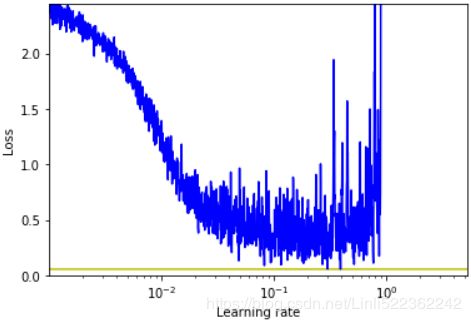
One way to find a good learning rate is to train the model for a few hundred iterations, starting with a very low learning rate (e.g., ) and gradually increasing it up to a very large value (e.g., 10). This is done by multiplying the learning rate by a constant factor at each iteration (e.g., by ) to go from to 10 in 500 iterations). If you plot the loss as a function of the learning rate (using a log scale for the learning rate), you should see it dropping at first. But after a while, the learning rate will be too large, so the loss will shoot back up: the optimal learning rate will be a bit lower than the point at which the loss starts to climb (typically about 10 times lower than the turning point). You can then reinitialize your model and train it normally using this good learning rate. We will look at more learning rate techniques in Chapter 11.

Optimizer

     Choosing a better optimizer than plain old Mini-batch Gradient Descent (and tuning its hyperparameters) is also quite important. We will see several advanced optimizers in Chapter 11.

Batch size

     The batch size can have a significant impact on your model’s performance and training time. The main benefit of using large batch sizes is that hardware accelerators like GPUs can process them efficiently (see Chapter 19), so the training algorithm will see more instances per second. Therefore, many researchers and practitioners recommend using the largest batch size that can fit in GPU RAM. There’s a catch, though: in practice, large batch sizes often lead to training instabilities, especially at the beginning of training, and the resulting model may not generalize as well as a model trained with a small batch size. In April 2018, Yann LeCun even tweeted “Friends don’t let friends use mini-batches larger than 32,” citing a 2018 paper by Dominic Masters and Carlo Luschi which concluded that using small batches (from 2 to 32) was preferable because small batches led to better models in less training time. Other papers point in the opposite direction, however; in 2017, papers by Elad Hoffer et al.25 and Priya Goyal et al.26 showed that it was possible to use very large batch sizes (up to 8,192) using various techniques such as warming up the learning rate (i.e., starting training with a small learning rate, then ramping it up, as we will see in Chapter 11). This led to a very short training time, without any generalization gap. So, one strategy is to try to use a large batch size, using learning rate warmup, and if training is unstable or the final performance is disappointing, then try using a small batch size instead.

Activation function

     We discussed how to choose the activation function earlier in this chapter: in general, the ReLU activation function will be a good default for all hidden layers. For the output layer, it really depends on your task.

Number of iterations

     In most cases, the number of training iterations does not actually need to be tweaked: just use early stopping instead.

     The optimal learning rate depends on the other hyperparameters—especially the batch size—so if you modify any hyperparameter, make sure to update the learning rate as well.

     For more best practices regarding tuning neural network hyperparameters, check out the excellent 2018 paper by Leslie Smith. This concludes our introduction to artificial neural networks and their implementation with Keras. In the next few chapters, we will discuss techniques to train very deep nets. We will also explore how to customize models using TensorFlow’s lowerlevel API and how to load and preprocess data efficiently using the Data API. And we will dive into other popular neural network architectures: convolutional neural networks for image processing, recurrent neural networks for sequential data, autoencoders for representation learning, and generative adversarial networks to model and generate data.

Exercises

1. The TensorFlow Playground is a handy neural network simulator built by the TensorFlow team. In this exercise, you will train several binary classifiers in just a few clicks, and tweak the model’s architecture and its hyperparameters to gain some intuition on how neural networks work and what their hyperparameters do. Take some time to explore the following: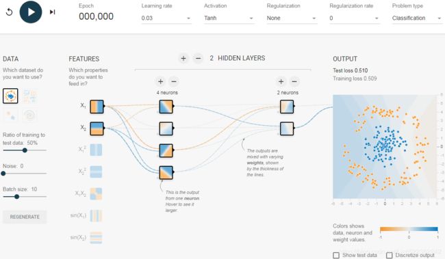

• a. The patterns learned by a neural net. Try training the default neural network by clicking the Run button (top left). Notice how it quickly finds a good solution for the classification task(100 epochs). The neurons in the first hidden layer have learned simple patterns, while the neurons in the second hidden layer have learned to combine the simple patterns of the first hidden layer into more complex patterns. In general, the more layers there are, the more complex the patterns can be.
  
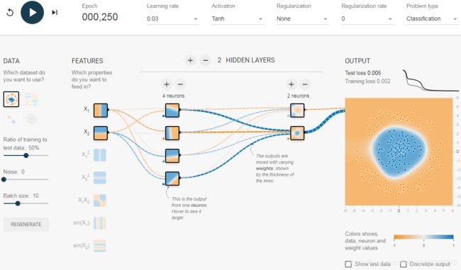
• b. Activation functions. Try replacing the tanh activation function with a ReLU activation function, and train the network again. Notice that it finds a solution even faster, but this time the boundaries are linear. This is due to the shape of the ReLU function.
  
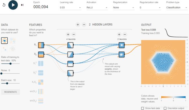
• c. The risk of local minima. Modify the network architecture to have just one hidden layer with three neurons. Train it multiple times (to reset the network weights, click the Reset button next to the Play button). Notice that the training time varies a lot, and sometimes it even gets stuck in a local minimum.
  
  
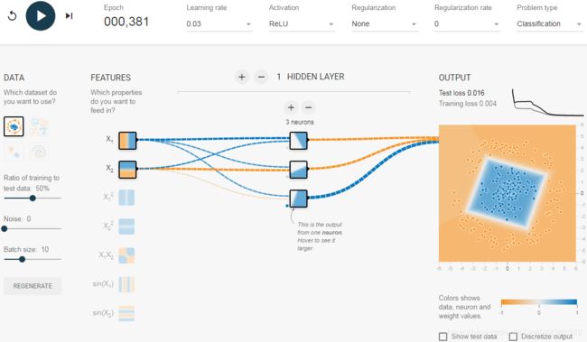
• d. What happens when neural nets are too small. Remove one neuron to keep just two. Notice that the neural network is now incapable of finding a good solution, even if you try multiple times. The model has too few parameters and systematically underfits the training set.
  
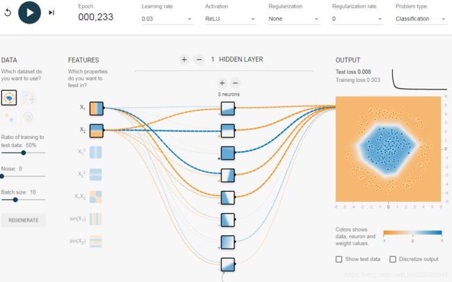
• e. What happens when neural nets are large enough. Set the number of neurons to eight, and train the network several times. Notice that it is now consistently fast and never gets stuck. This highlights an important finding in neural network theory: large neural networks almost never get stuck in local minima, and even when they do these local optima are almost as good as the global optimum. However, they can still get stuck on long plateaus for a long time.
  
• f. The risk of vanishing gradients in deep networks. Select the spiral螺旋 dataset (the bottom-right dataset under “DATA”), and change the network architecture to have four hidden layers with eight neurons each. Notice that training takes much longer and often gets stuck on plateaus高原 for long periods of time. Also notice that the neurons in the highest layers (on the right) tend to evolve faster than the neurons in the lowest layers (on the left). This problem, called the “vanishing gradients” problem, can be alleviated减轻的 with better weight initialization and other techniques, better optimizers (such as AdaGrad or Adam), or Batch Normalization (discussed in Chapter 11).
  
• g. Go further. Take an hour or so to play around with other parameters and get a feel for what they do, to build an intuitive understanding about neural networks.https://playground.tensorflow.org/#activation=relu®ularization=L2&batchSize=10&dataset=spiral®Dataset=reg-plane&learningRate=0.03®ularizationRate=0&noise=0&networkShape=8,8,8,8&seed=0.58750&showTestData=false&discretize=false&percTrainData=50&x=true&y=true&xTimesY=false&xSquared=true&ySquared=true&cosX=false&sinX=false&cosY=false&sinY=false&collectStats=false&problem=classification&initZero=false&hideText=false

2. Draw an ANN using the original artificial neurons (like the ones in Figure 10-3) that computes A ⊕ B (where ⊕ represents the XOR operation). Hint: A ⊕ B = (A ∧ ¬ B ∨ (¬ A ∧ B).

3. Why is it generally preferable to use a Logistic Regression classifier rather than a classical Perceptron (i.e., a single layer of threshold logic units trained using the Perceptron training algorithm)? How can you tweak a Perceptron to make it equivalent to a Logistic Regression classifier?
Perceptron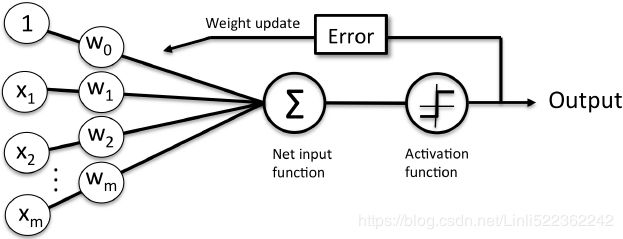

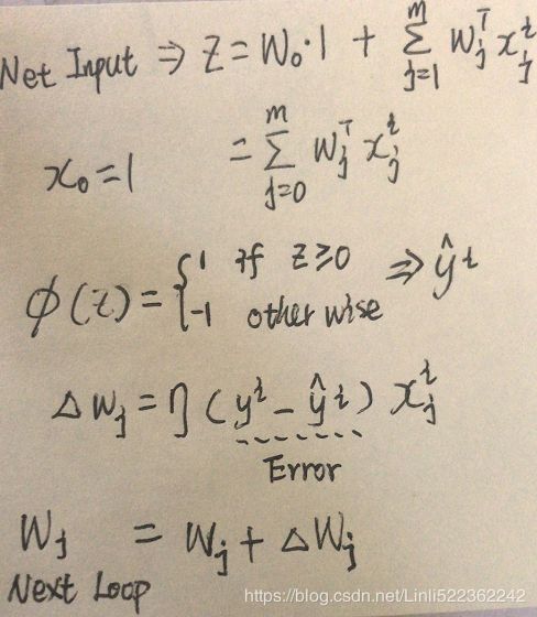
     A classical Perceptron will converge only if the dataset is linearly separable, and it won’t be able to estimate class probabilities. In contrast, a Logistic Regression classifier will converge to a good solution even if the dataset is not linearly separable, and it will output class probabilities. If you change the Perceptron’s activation function to the logistic activation function (or the softmax activation function if there are multiple neurons), and if you train it using Gradient Descent (or some other optimization algorithm minimizing the cost function, typically cross entropy), then it becomes equivalent to a Logistic Regression classifier.

Equation 4-19. Softmax score for class k  

Equation 4-20. Softmax function 
Equation 4-21. Softmax Regression classifier prediction 

Equation 4-22. Cross entropy cost function 
 is equal to 1 if the target class for the ith instance is k; otherwise, it is equal to 0.

4. Why was the logistic activation function a key ingredient成分 in training the first MLPs?

     The logistic activation function was a key ingredient in training the first MLPs because its derivative is always nonzero, so Gradient Descent can always roll down the slope. When the activation function is a step function, Gradient Descent cannot move, as there is no slope at all.
     

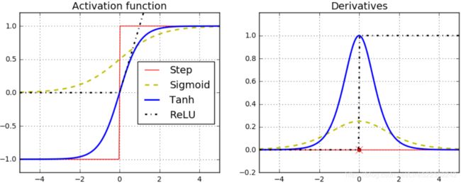
5. Name three popular activation functions. Can you draw them?

     Popular activation functions include the step function, the logistic (sigmoid) function, the hyperbolic tangent (tanh) function, and the Rectified Linear Unit (ReLU) function (see Figure 10-8). See Chapter 11 for other examples, such as ELU and variants of the ReLU function.

6. Suppose you have an MLP composed of one input layer with 10 passthrough neurons, followed by one hidden layer with 50 artificial neurons, and finally one output layer with 3 artificial neurons. All artificial neurons use the ReLU activation function.

• What is the shape of the input matrix X?
       The shape of the input matrix X is m × 10, where m represents the training batch size.
• What are the shapes of the hidden layer’s weight vector and its bias vector ?
       The shape of the hidden layer’s weight vector is 10 × 50 and the length of its bias vector is 50.
• What are the shapes of the output layer’s weight vector and its bias vector ?
       The shape of the output layer’s weight vector is 50 × 3, and the length of its bias vector is 3.
• What is the shape of the network’s output matrix Y?
       The shape of the network’s output matrix Y is m × 3.
• Write the equation that computes the network’s output matrix Y as a function of X, , , , and .
   Note that when you are adding a bias vector to a matrix, it is added to every single row in the matrix, which is called broadcasting.

7. How many neurons do you need in the output layer if you want to classify email into spam or ham? What activation function should you use in the output layer? If instead you want to tackle MNIST, how many neurons do you need in the output layer, and which activation function should you use? What about for getting your network to predict housing prices, as in Chapter 2?

     To classify email into spam or ham, you just need one neuron in the output layer of a neural network—for example, indicating the probability that the email is spam. You would typically use the logistic activation function in the output layer
when estimating a probability. If instead you want to tackle MNIST, you need 10 neurons in the output layer, and you must replace the logistic function with the softmax activation function, which can handle multiple classes, outputting one probability per class. Now, if you want your neural network to predict housing prices like in Chapter 2, then you need one output neuron, using no activation function at all in the output layer.

8. What is backpropagation and how does it work? What is the difference between backpropagation and reverse-mode autodiff?
     Backpropagation反向传播(B-P网络) is a technique used to train artificial neural networks. It first computes the gradients of the cost function with regard to every model parameter (all the weights and biases), then it performs a Gradient Descent step using these gradients. This backpropagation step is typically performed thousands or millions of times, using many training batches, until the model parameters converge to values that (hopefully) minimize the cost function. To compute the gradients, backpropagation uses reverse-mode autodiff (although it wasn’t called that when backpropagation was invented, and it has been reinvented several times).

f(x,y)=with regards to x at x = 3 and y = 4 ,  f =  and Since  simply performs the sum =, we find that , so   .
==>
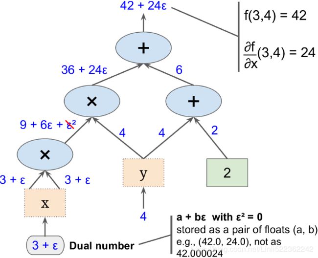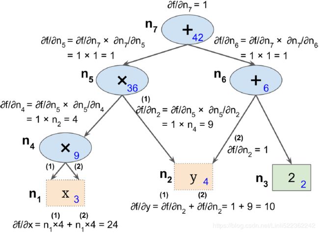
Figure D-2. Forward-mode autodiff                    Figure D-3. Reverse-mode autodiff
     Reverse-mode autodiff performs a forward pass through a computation graph, computing every node’s value for the current training batch, and then it performs a reverse pass, computing all the gradients at once (see https://blog.csdn.net/Linli522362242/article/details/106290394 for more details). So what’s the difference? Well, backpropagation refers to the whole process of training an artificial neural network using multiple backpropagation steps, each of which computes gradients and uses them to perform a Gradient Descent step. In contrast, reverse-mode autodiff is just a technique to compute gradients efficiently, and it happens to be used by backpropagation.

9. Can you list all the hyperparameters you can tweak in a basic MLP? If the MLP overfits the training data, how could you tweak these hyperparameters to try to solve the problem?

     Here is a list of all the hyperparameters you can tweak in a basic MLP: the number of hidden layers, the number of neurons in each hidden layer, and the activation function used in each hidden layer and in the output layer. In general, the ReLU activation function (or one of its variants; see Chapter 11) is a good default for the hidden layers. For the output layer, in general you will want the logistic activation function for binary classification, the softmax activation function for multiclass classification, or no activation function for regression.

     If the MLP overfits the training data, you can try reducing the number of hidden layers and reducing the number of neurons per hidden layer.

10. Train a deep MLP on the MNIST dataset (you can load it using keras.data sets.mnist.load_data(). See if you can get over 98% precision. Try searching for the optimal learning rate by using the approach presented in this chapter (i.e., by growing the learning rate exponentially, plotting the loss, and finding the point where the loss shoots up). Try adding all the bells and whistles—save checkpoints, use early stopping, and plot learning curves using TensorBoard.

 

Let's load the dataset:

from tensorflow import keras

(x_train_full, y_train_full), (x_test, y_test) = keras.datasets.mnist.load_data()

Just like for the Fashion MNIST dataset, the MNIST training set contains 60,000 grayscale images, each 28x28 pixels: 

x_train_full.shape, y_train_full.shape, x_test.shape, y_test.shape

 
Each pixel intensity is also represented as a byte (0 to 255):

x_train_full.dtype

 
     Let's split the full training set into a validation set and a (smaller) training set. We also scale the pixel intensities down to the 0-1 range and convert them to floats, by dividing by 255, just like we did for Fashion MNIST:

# the original dtype=unit8, now it will be converted to np.float32 
# For simplicity, we’ll scale the pixel intensities down to the 0–1 range by dividing them by 255.0 
x_valid, x_train = x_train_full[:5000] /255., x_train_full[5000:]/255.
y_valid, y_train = y_train_full[:5000], y_train_full[5000:]
x_test = x_test/255.

 

Let's plot an image using Matplotlib's imshow() function, with a 'binary' color map:

import matplotlib.pyplot as plt

plt.imshow(x_train[0], cmap="binary")
plt.axis('off')
plt.show()

 

     The labels are the class IDs (represented as uint8), from 0 to 9. Conveniently, the class IDs correspond to the digits represented in the images, so we don't need a class_names array:

y_train

 
The validation set contains 5,000 images, and the test set contains 10,000 images:

x_valid.shape

 

Let's take a look at a sample of the images in the dataset:

n_rows = 4
n_cols = 10

plt.figure( figsize=(n_cols*1.2, n_rows*1.2) )

for row in range(n_rows):
    for col in range(n_cols):
        index = n_cols * row + col
        plt.subplot( n_rows, n_cols, index+1 ) # the subplot's index start 1
        plt.imshow(x_train[index], cmap="binary", interpolation="nearest" )
        plt.axis("off") #remove the axis
        plt.title(y_train[index], fontsize=12)

plt.subplots_adjust(wspace=0.2, hspace=0.5)
plt.show()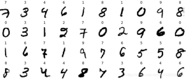

 
Try searching for the optimal learning rate by using the approach presented in this chapter (i.e., by growing the learning rate exponentially, plotting the loss, and finding the point where the loss shoots up)

     Let's build a simple dense network and find the optimal learning rate. We will need a callback to grow the learning rate at each iteration. It will also record the learning rate and the loss at each iteration:

K = keras.backend

class ExponentialLearningRate( keras.callbacks.Callback ):################################
    def __init__(self, factor):
        self.factor = factor
        self.rates = []
        self.losses = []
    def on_batch_end(self, batch, logs):
        self.rates.append( K.get_value(self.model.optimizer.lr) )
        self.losses.append( logs['loss'] )
                    #(tensor,                    value)
        K.set_value( self.model.optimizer.lr, self.model.optimizer.lr*self.factor)########

keras.backend.clear_session()
import numpy as np
np.random.seed(42)
import tensorflow as tf
tf.random.set_seed(42)

n_hidden1 = 300
n_hidden2 = 100
n_outputs = 10

model = keras.models.Sequential([
    # It is a Flatten layer whose role is to convert each input image into a 1D array
    keras.layers.Flatten(input_shape=[28,28]), #to 28*28=784 neurons
    keras.layers.Dense(n_hidden1, activation='relu', name="hidden1"),
    keras.layers.Dense(n_hidden2, activation='relu', name='hidden2' ),
    keras.layers.Dense(n_outputs, activation='softmax', name='output')
])

 

We will start with a small learning rate of 1e-3, and grow it by 0.5% at each iteration:

model.compile( loss="sparse_categorical_crossentropy",
               optimizer=keras.optimizers.SGD(lr=1e-3),
               metrics=['accuracy']
             )
expon_lr = ExponentialLearningRate(factor=1.005)

 Now let's train the model for just 1 epoch:

history = model.fit( x_train, y_train, epochs=1, 
                     validation_data=(x_valid, y_valid),
                     callbacks=[expon_lr] ################
                   )

 

 We can now plot the loss as a functionof the learning rate:

plt.plot(expon_lr.rates, expon_lr.losses, color='b')
plt.gca().set_xscale('log')############
plt.hlines( min(expon_lr.losses),  #y
            min(expon_lr.rates),   #xmin
            max(expon_lr.rates),   #xmax
            color='y' )
plt.axis([ min(expon_lr.rates), max(expon_lr.rates), 
          0, expon_lr.losses[0] ])
plt.xlabel("Learning rate")
plt.ylabel("Loss")
plt.show()

 ==>

The loss starts shooting back up violently around 3e-1, so let's try using 2e-1 as our learning rate: 

keras.backend.clear_session()
np.random.seed(42)
tf.random.set_seed(42)

n_hidden1 = 300
n_hidden2 = 100
n_outputs = 10

model = keras.models.Sequential([
    # It is a Flatten layer whose role is to convert each input image into a 1D array
    keras.layers.Flatten(input_shape=[28,28]), #to 28*28=784 neurons
    keras.layers.Dense(n_hidden1, activation='relu', name="hidden1"),
    keras.layers.Dense(n_hidden2, activation='relu', name='hidden2' ),
    keras.layers.Dense(n_outputs, activation='softmax', name='output')
])

model.compile( loss="sparse_categorical_crossentropy",
               optimizer=keras.optimizers.SGD(lr=2e-1),##################
               metrics=['accuracy']
             )

run_index = 1 # increment this at every run
import os
                                                     #fill with 0, 3 digits after '.', integer~d
run_logdir = os.path.join( os.curdir, "my_mnist_logs", "run{:03d}".format(run_index) )
run_logdir

 

early_stopping_cb = keras.callbacks.EarlyStopping(patience=20)
checkpoint_cb = keras.callbacks.ModelCheckpoint("my_mnist_model.h5", save_best_only=True)
tensorboard_cb = keras.callbacks.TensorBoard(run_logdir)

history = model.fit(x_train, y_train, epochs=100,
                    validation_data=(x_valid, y_valid),
                    callbacks=[early_stopping_cb, checkpoint_cb, tensorboard_cb]
                   )

... ... 

model = keras.models.load_model("my_mnist_model.h5") # rollback to best model
model.evaluate(x_test, y_test)

 
We got  98% accuracy. Finally, let's look at the learning curves using TensorBoard:

%load_ext tensorboard
%tensorboard --logdir=./my_mnist_logs --port=6006