目标检测(YOLO,FPN,RetinaNet,SSD)

在前一篇目标检测(R-CNN,SPP,Fast R-CNN,Faster R-CNN),所整理的R-CNN,SPP,Fast R-CNN,Faster R-CNN中,这些目标检测技术都只是两阶段网络,比如性能相对来说最好的Faster R-CNN,是先用RPN生成候选目标区域,然后再进行Fast R-CNN的方法,继续目标对象的分类和边框的回归预测。但是那有办法一步做完这些事吗?
YOLO
YOLO是一个很重要的目标检测框架,准确率和检测速度都非常好也已经进化更新了3代了(https://pjreddie.com/media/files/papers/YOLOv3.pdf)。它之所以可以一步到位,就是使用了如下图的统一架构:

即先把图片分成固定的单元S x S,如图是7 X 7,每个方格都各自负责使用卷积去预测框内有无目标存在的情况,再以小格子为中心寻找更精确的目标框,如图中各种颜色的预测,最后再结合预测到的概率,最大化抑制等就可以得到最后的结果。即它的检测过程是:
1.划分方格,每个方格有(x,y,w,h,confidence,C1…Cn),(x,y)坐标代表了中心,w,h分别代表目标的宽度高度比(相对整张图),置信度是由预测框和任意实际框的iou值,C是预测到的类别,用这样的矩阵格式就可以一次性的预测出类别,边框。因此对于有10个类别的数据来说,每个方格使用2种大小的锚框(一宽一窄),那么每个方格单元的输出将会是((4+1)2+10)=20,那么对于77的方格数,最后有7720大小的的输出。
2.输入到网络中进行训练。如下图是YOLO自己所使用了一种叫DarkNet的网络。

损失函数:

Yolo损失函数一共包括:协调误差,客体性的分数( 1 o b j 1^{obj} 1obj,评价框内是否存在目标,只有它大于0.5时,才有计算协调误差和分类误差),分类误差三项。其中第一项是边界框中心坐标的误差项, 1 o b j 1^{obj} 1obj指的是第i个单元格存在目标,而且该单元格中的第j个边界框负责预测该目标。第二项是边界框的高与宽的W,H误差项。第三项是包含目标的边界框的置信度误差项。第四项是不包含目标的边界框的置信度误差项。而最后一项是包含目标的单元格的分类误差项, 1 o b j 1^{obj} 1obj指的是第i个单元格存在目标。但是实际上这个误差函数并不是对所以的数据集都适用,在其他的数据上它的效果可能并没有那么的出色。
YOLO的全项目地址是:https://pjreddie.com/darknet/ ,下面是部分代码解析:
#YOLO网络模型
from keras.models import Model
from keras.layers import Input, Conv2D, GlobalAveragePooling2D, Dense
from keras.layers import add, Activation, BatchNormalization
from keras.layers.advanced_activations import LeakyReLU
from keras.regularizers import l2

#每个卷积层
def conv2d_unit(x, filters, kernels, strides=1):
    x = Conv2D(filters, kernels,
               padding='same',
               strides=strides,
               activation='linear',
               kernel_regularizer=l2(5e-4))(x)
    x = BatchNormalization()(x)#BN处理
    x = LeakyReLU(alpha=0.1)(x)#使用LeakyReLU做激活函数

    return x

#每个残差块
def residual_block(inputs, filters):
    x = conv2d_unit(inputs, filters, (1, 1))
    x = conv2d_unit(x, 2 * filters, (3, 3))
    x = add([inputs, x])
    x = Activation('linear')(x)

    return x

#一堆残差块
def stack_residual_block(inputs, filters, n):
    x = residual_block(inputs, filters)

    for i in range(n - 1):
        x = residual_block(x, filters)

    return x

#darknet架构
def darknet_base(inputs):
    x = conv2d_unit(inputs, 32, (3, 3))

    x = conv2d_unit(x, 64, (3, 3), strides=2)
    x = stack_residual_block(x, 32, n=1)

    x = conv2d_unit(x, 128, (3, 3), strides=2)
    x = stack_residual_block(x, 64, n=2)

    x = conv2d_unit(x, 256, (3, 3), strides=2)
    x = stack_residual_block(x, 128, n=8)

    x = conv2d_unit(x, 512, (3, 3), strides=2)
    x = stack_residual_block(x, 256, n=8)

    x = conv2d_unit(x, 1024, (3, 3), strides=2)
    x = stack_residual_block(x, 512, n=4)

    return x


def darknet():
    inputs = Input(shape=(416, 416, 3))
    x = darknet_base(inputs)

    x = GlobalAveragePooling2D()(x)#全局平均池化以处理size不一致(改进SPP的池化方法)
    x = Dense(1000, activation='softmax')(x)

    model = Model(inputs, x)

    return model


if __name__ == '__main__':
    model = darknet()
    print(model.summary())
#YOLOv3的处理模式
import numpy as np
import keras.backend as K
from keras.models import load_model

class YOLO:
    def __init__(self, obj_threshold, nms_threshold):
        self._t1 = obj_threshold#目标置信度阈值
        self._t2 = nms_threshold#非极大抑制阈值
        self._yolo = load_model('data/yolo.h5')#预训练结束的YOLO模型

    def _sigmoid(self,x):
        return 1 / (1 + np.exp(-x))

   #特征处理,即处理网络所输出的矩阵【x,y,w,h,confidence,C....】
    def _process_feats(self, out, anchors, mask):
        grid_h, grid_w, num_boxes = map(int, out.shape[1: 4])#得到输出的h,w,和锚框数

        anchors = [anchors[i] for i in mask]#mask是锚框形态
        # 重新处理各数据的排列
        out = out[0]
        box_xy = self._sigmoid(out[..., :2])
        box_wh = np.exp(out[..., 2:4])
        box_wh = box_wh * anchors
        box_confidence = self._sigmoid(out[..., 4])
        box_confidence = np.expand_dims(box_confidence, axis=-1)#加入一列
        box_class_probs = self._sigmoid(out[..., 5:])#类别预测值

        col = np.tile(np.arange(0, grid_w), grid_w).reshape(-1, grid_w)
        row = np.tile(np.arange(0, grid_h).reshape(-1, 1), grid_h)

        col = col.reshape(grid_h, grid_w, 1, 1).repeat(3, axis=-2)
        row = row.reshape(grid_h, grid_w, 1, 1).repeat(3, axis=-2)
        grid = np.concatenate((col, row), axis=-1)

        box_xy += grid
        box_xy /= (grid_w, grid_h)
        box_wh /= (416, 416)
        box_xy -= (box_wh / 2.)
        boxes = np.concatenate((box_xy, box_wh), axis=-1)#拼接成每个框的xywh

        return boxes, box_confidence, box_class_probs

   #目标置信度阈值t1过滤框
    def _filter_boxes(self, boxes, box_confidences, box_class_probs):
        box_scores = box_confidences * box_class_probs
        box_classes = np.argmax(box_scores, axis=-1)
        box_class_scores = np.max(box_scores, axis=-1)
        pos = np.where(box_class_scores >= self._t1)

        boxes = boxes[pos]
        classes = box_classes[pos]
        scores = box_class_scores[pos]

        return boxes, classes, scores

  #非极大抑制阈值t2过滤框
    def _nms_boxes(self, boxes, scores):
        x = boxes[:, 0]
        y = boxes[:, 1]
        w = boxes[:, 2]
        h = boxes[:, 3]

        areas = w * h
        order = scores.argsort()[::-1]

        keep = []
        while order.size > 0:
            i = order[0]
            keep.append(i)

            xx1 = np.maximum(x[i], x[order[1:]])
            yy1 = np.maximum(y[i], y[order[1:]])
            xx2 = np.minimum(x[i] + w[i], x[order[1:]] + w[order[1:]])
            yy2 = np.minimum(y[i] + h[i], y[order[1:]] + h[order[1:]])

            w1 = np.maximum(0.0, xx2 - xx1 + 1)
            h1 = np.maximum(0.0, yy2 - yy1 + 1)
            inter = w1 * h1

            ovr = inter / (areas[i] + areas[order[1:]] - inter)
            inds = np.where(ovr <= self._t2)[0]
            order = order[inds + 1]

        keep = np.array(keep)

        return keep#最好的锚框

    def _yolo_out(self, outs, shape):
        masks = [[6, 7, 8], [3, 4, 5], [0, 1, 2]]#用于指定anchors的形态组
        anchors = [[10, 13], [16, 30], [33, 23], [30, 61], [62, 45],
                   [59, 119], [116, 90], [156, 198], [373, 326]]

        boxes, classes, scores = [], [], []

        for out, mask in zip(outs, masks):
            b, c, s = self._process_feats(out, anchors, mask)#输出的标准预测矩阵
            b, c, s = self._filter_boxes(b, c, s)#过滤掉置信度不够的锚框
            boxes.append(b)
            classes.append(c)
            scores.append(s)

        boxes = np.concatenate(boxes)
        classes = np.concatenate(classes)
        scores = np.concatenate(scores)

        # Scale boxes back to original image shape.
        width, height = shape[1], shape[0]
        image_dims = [width, height, width, height]
        boxes = boxes * image_dims

        nboxes, nclasses, nscores = [], [], []
        for c in set(classes):#对每个预测出的种类
            inds = np.where(classes == c)
            b = boxes[inds]
            c = classes[inds]
            s = scores[inds]

            keep = self._nms_boxes(b, s)#去除重合的锚框

            nboxes.append(b[keep])
            nclasses.append(c[keep])
            nscores.append(s[keep])

        if not nclasses and not nscores:
            return None, None, None

        boxes = np.concatenate(nboxes)
        classes = np.concatenate(nclasses)
        scores = np.concatenate(nscores)

        return boxes, classes, scores

    def predict(self, image, shape):
        outs = self._yolo.predict(image)
        boxes, classes, scores = self._yolo_out(outs, shape)

        return boxes, classes, scores
此后还有很多借鉴了这种结构的算法如FRN,RetinaNet。
FPN
特征金字塔网络(Feature Pyramid networks, FPN)主要解决的问题就是对小物体的难以捕捉问题。如下图的图像金字塔结构,把缩放(通过采样和插值等方法)到不同尺寸的图像输入到网络中,每个尺寸的图像一旦被检测器检测到,再使用不同的方式结合所有预测到的结果。这一技术也可以跟R-CNN,Fast R-CNN结合能到更好的效果。

RetinaNet
RetinaNet主要解决的问题就是一步做完却会导致的----类别不平衡问题,即在得到的一堆锚框中,实际上只有少数量的目标框,还有很多无用的背景图,导致极端的类别不平衡。在Faster R-CNN,由于使用了RPN,它会先对锚框进行简单的二分类(区分是前景目标还是背景,但是并不会区别究竟属于哪个细类,这是后面的类别判断器会做的预测),这样会减少很多无用的背景框,提升精度。
所以它采用的方法就是回归任务的交叉熵误差改为焦点损失 FL (focal loss) 函数:
F L ( p t ) = − ( 1 − p t ) γ log ( p t ) = ( 1 − p t ) γ C E ( y ^ ) i FL(p_t) = -(1-p_t)^\gamma \log(p_t) = (1-p_t)^\gamma CE(\hat{y})_{i} FL(pt)=−(1−pt)γlog(pt)=(1−pt)γCE(y^)i
此处的 P t P_{t} Pt取值为,如果y=1,则为p,否则为1-p。α 叫做平衡参数(特定类实例数的倒数,即1/n)和 γ 叫聚焦参数。
其中可以看到CE就是原交叉熵 C E ( p t ) = − α t log ( p t ) CE(p_t)=-\alpha_t \log(p_t) CE(pt)=−αtlog(pt),相较之下就是多加入了一个权重 ( 1 − p t ) γ (1-p_t)^\gamma (1−pt)γ,加入了这个权重后,它可以为具有更多样本的背景类提供了较少的权重,所以相当于给数量少的类增加了权重。比如:
1容易分类
容易分类的前景目标p=0.9。
交叉熵:是CE(前景)=-log(0.9)=0.1053
焦点损失(使用alpha=0.25和gamma=2):FL(前景)=-1 x 0.25 x(1–0.9)**2log(0.9)=0.00026
容易分类的背景目标p=0.1。
E(背景)=-log(1–0.1)=0.1053
FL(背景)=-1 x 0.25 x(1–(1–0.1))**2log(1–0.1)=0.00026。
2.错误分类
错误分类的前景目标p=0.1。
CE(前景)=-log(0.1)=2.3025
FL(前景)=-1 x 0.25 x(1–0.1)**2log(0.1)=0.4667
错误分类背景目标P=0.9。
CE(背景)=-log(1–0.9)=2.3025
FL(背景)=-1 x 0.25 x(1–(1–0.9))**2log(1–0.9)=0.4667
相比之下容易分类的产生的loss从0.1变成了0.00026这么小的数,而错误分类则减少了5倍,相对来说会使模型更加的注重不好区分的场景,同时对于数量大的背景图来说,减少的权重要远多于数量少的目标图,这样就相当于给目标框加了权重,从而解决了样本不平衡问题。
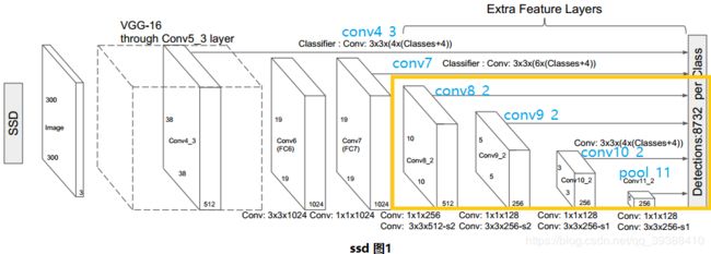
SSD
与YOLO的区别主要就是在做目标检测时,不仅仅使用最后得到的特征图上,还在网络的前几层5个特征图上也进行预测,即多尺度融合。如下图中全部都输入到了最后一层。这样能保证对小物体的识别精度(克服YOLO7X7太粗糙)。
使用JacCard重叠,所有重叠大于0.5的锚定箱均视为正例。使用的损失函数为:
L ( x , c , l , g ) = 1 N ( L c o n f ( x , c ) + α L l o c ( x , l , g ) ) L(x,c,l,g)=\frac {1}{N} (L_{conf}(x,c)+\alpha L_{loc}(x,l,g)) L(x,c,l,g)=N1(Lconf(x,c)+αLloc(x,l,g))
对于置信度,使用交叉熵损失。对于loc,使用平滑的L1损失。为了解决类别不平衡,不是随机抽取训练而是对反样本(背景)按降序排列了他们的“反对”分数,然后再反:正3:1采样。
为什么对小目标预测效果不好?
小目标对应的anchor会很少,而在检测目标时,需要足够大的feature map来提供精确特征,同时也需要足够的语义信息来将其与背景做区分。
TensorFlow Object Detection API
前一篇的目标检测(R-CNN,SPP,Fast R-CNN,Faster R-CNN),中有用Tensorflow的目标检测API,使用它已经训练好的SSD + MobileNet网络做自己图片目标检测的测试。那么如何训练一个自己的网络?
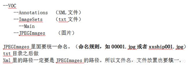
1.数据集使用VOC2012(也自然可以使用自己的数据集, 图片用LabelImg标注后,做成VOC的形式)。
2.将VOC转为tfrecord形式,并存为pascal_的名字。
python create_pascal_tf_record.py --data_dir voc/ --year= VOC2012 --set=train --output_path=voc/pascal_train.record
python create_pascal_tf_record.py --data_dir voc/ --year= VOC2012 --set=val --output_path=voc/pascal_val.record
3.复制pascal_label_map到voc文件夹下。
cp data/pascal_label_map.pbtxt voc/
4.网络的训练需要设置一些配置文件的辅助来实现,所以先复制所需要的网络架构的配置文件如faster_rcnn_inception_resnet_v2_atrous_pets.config到voc路径下。
5.修改预训练网络的配置文件,即打开或之前下载任意预训练网络的模型参数如ssd_mobilenet_v1_coco.config配置文件,分类数num_classes如voc2012是20类;num_examples表示测试时的图片数量如voc2012是5823;还有就是几处PATH_TO_BE_CONFIGURED的路径改成voc下相应的数据路径。
6.在voc下新建一个train_dir作为保存模型和日志的目录。
7.开始训练网络
python train.py --logtostderr --train_dir=voc/train_dir/ --pipeline_config_path=voc/train_dir/ssd_mobilenet_v1_coco.config
8.可视化
tensorboard --logdir='train_dir'
9 等训练完成后,就可以开始测试训练的情况了,其中1000只是指第1000步的结果
python export_inference_graph.py --input_type image_tensor \--pipeline_config_path.voc/voc.config\--trained_checkpoint_prefix voc/train_dir/model .ckpt-1000 --output_directory voc/export/
就可以得到最后的训练结果。
