感知机算法
《统计学习方法》系列笔记的第二篇,对应原著第二章。大量引用原著讲解,加入了自己的理解。对书中算法采用Python实现,并用Matplotlib可视化了动画出来,应该算是很硬派了。一套干货下来,很是辛苦,要是能坚持下去就好。
概念
感知机是二分类模型,输入实例的特征向量,输出实例的±类别。
感知机模型
定义
假设输入空间是x和y分属这两个空间,那么由输入空间到输出空间的如下函数:
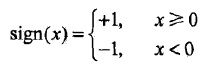
叫做偏置,w·x表示向量w和x的内积。sign是一个函数:
感知机的几何解释是,线性方程
将特征空间划分为正负两个部分:

这个平面(2维时退化为直线)称为分离超平面。
感知机学习策略
数据集的线性可分性
定义
给定数据集
如果存在某个超平面S
能够完全正确地将正负实例点全部分割开来,则称T线性可分,否则称T线性不可分
感知机学习策略
假定数据集线性可分,我们希望找到一个合理的损失函数。
一个朴素的想法是采用误分类点的总数,但是这样的损失函数不是参数w,b的连续可导函数,不可导自然不能把握函数的变化,也就不易优化(不知道什么时候该终止训练,或终止的时机不是最优的)。
另一个想法是选择所有误分类点到超平面S的总距离。为此,先定义点x0到平面S的距离:

是w的L2范数,所谓L2范数,指的是向量各元素的平方和然后求平方根(长度)。这个式子很好理解,回忆中学学过的点到平面的距离:
此处的点到超平面S的距离的几何意义就是上述距离在多维空间的推广。
又因为,如果点i被误分类,一定有
成立,所以我们去掉了绝对值符号,得到误分类点到超平面S的距离公式:

假设所有误分类点构成集合M,那么所有误分类点到超平面S的总距离为
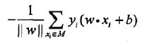
分母作用不大,反正一定是正的,不考虑分母,就得到了感知机学习的损失函数:
感知机学习算法
原始形式
感知机学习算法是对以下最优化问题的算法:
感知机学习算法是误分类驱动的,先随机选取一个超平面,然后用梯度下降法不断极小化上述损失函数。损失函数的梯度由:
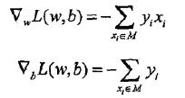
给出。所谓梯度,是一个向量,指向的是标量场增长最快的方向,长度是最大变化率。所谓标量场,指的是空间中任意一个点的属性都可以用一个标量表示的场(个人理解该标量为函数的输出)。
随机选一个误分类点i,对参数w,b进行更新:
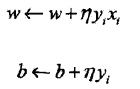
是学习率。损失函数的参数加上梯度上升的反方向,于是就梯度下降了。所以,上述迭代可以使损失函数不断减小,直到为0。于是得到了原始形式的感知机学习算法:
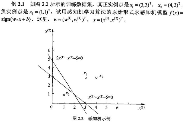
对于此算法,使用下面的例子作为测试数据:
给出Python实现和可视化代码如下:
终于到了最激动人心的时刻了,有了上述知识,就可以完美地可视化这个简单的算法:
    import copy
    from matplotlib import pyplot as plt
    from matplotlib import animation

    training_set = [[(3, 3), 1], [(4, 3), 1], [(1, 1), -1]]
    w = [0, 0]
    b = 0
    history = []


    def update(item):
        """
        update parameters using stochastic gradient descent
        :param item: an item which is classified into wrong class
        :return: nothing
        """
        global w, b, history
        w[0] += 1 * item[1] * item[0][0]
        w[1] += 1 * item[1] * item[0][1]
        b += 1 * item[1]
        print w, b
        history.append([copy.copy(w), b])
        # you can uncomment this line to check the process of stochastic gradient descent


    def cal(item):
        """
        calculate the functional distance between 'item' an the dicision surface. output yi(w*xi+b).
        :param item:
        :return:
        """
        res = 0
        for i in range(len(item[0])):
            res += item[0][i] * w[i]
        res += b
        res *= item[1]
        return res


    def check():
        """
        check if the hyperplane can classify the examples correctly
        :return: true if it can
        """
        flag = False
        for item in training_set:
            if cal(item) <= 0:
                flag = True
                update(item)
        # draw a graph to show the process
        if not flag:
            print "RESULT: w: " + str(w) + " b: " + str(b)
        return flag


    if __name__ == "__main__":
        for i in range(1000):
            if not check(): break

        # first set up the figure, the axis, and the plot element we want to animate
        fig = plt.figure()
        ax = plt.axes(xlim=(0, 2), ylim=(-2, 2))
        line, = ax.plot([], [], 'g', lw=2)
        label = ax.text([], [], '')

        # initialization function: plot the background of each frame
        def init():
            line.set_data([], [])
            x, y, x_, y_ = [], [], [], []
            for p in training_set:
                if p[1] > 0:
                    x.append(p[0][0])
                    y.append(p[0][1])
                else:
                    x_.append(p[0][0])
                    y_.append(p[0][1])

            plt.plot(x, y, 'bo', x_, y_, 'rx')
            plt.axis([-6, 6, -6, 6])
            plt.grid(True)
            plt.xlabel('x')
            plt.ylabel('y')
            plt.title('Perceptron Algorithm (www.hankcs.com)')
            return line, label


        # animation function.  this is called sequentially
        def animate(i):
            global history, ax, line, label

            w = history[i][0]
            b = history[i][1]
            if w[1] == 0: return line, label
            x1 = -7
            y1 = -(b + w[0] * x1) / w[1]
            x2 = 7
            y2 = -(b + w[0] * x2) / w[1]
            line.set_data([x1, x2], [y1, y2])
            x1 = 0
            y1 = -(b + w[0] * x1) / w[1]
            label.set_text(history[i])
            label.set_position([x1, y1])
            return line, label

        # call the animator.  blit=true means only re-draw the parts that have changed.
        print history
        anim = animation.FuncAnimation(fig, animate, init_func=init, frames=len(history), interval=1000, repeat=True,
                                       blit=True)
        plt.show()
        anim.save('perceptron.gif', fps=2, writer='imagemagick')
可视化

可见超平面被误分类点所吸引,朝着它移动,使得两者距离逐步减小,直到正确分类为止。通过这个动画,是不是对感知机的梯度下降算法有了更直观的感悟呢?
算法的收敛性
记输入向量加进常数1的拓充形式的超平面可以将数据集完全正确地分类,定义最小值伽马:
感知机学习算法的对偶形式
对偶指的是,将w和b表示为测试数据i的线性组合形式,通过求解系数得到w和b。具体说来,如果对误分类点i逐步修改wb修改了n次,则w,b关于i的增量分别为,则最终求解到的参数分别表示为:

于是有算法2.2:
则误分类次数k满足:

证明请参考《统计学习方法》P31。
感知机对偶算法代码
涉及到比较多的矩阵计算,于是用NumPy比较多:
    # -*- coding:utf-8 -*-
    # Filename: train2.2.py
    # Author:hankcs
    # Date: 2015/1/31 15:15
    import numpy as np
    from matplotlib import pyplot as plt
    from matplotlib import animation

    # An example in that book, the training set and parameters' sizes are fixed
    training_set = np.array([[[3, 3], 1], [[4, 3], 1], [[1, 1], -1]])

    a = np.zeros(len(training_set), np.float)
    b = 0.0
    Gram = None
    y = np.array(training_set[:, 1])
    x = np.empty((len(training_set), 2), np.float)
    for i in range(len(training_set)):
        x[i] = training_set[i][0]
    history = []

    def cal_gram():
        """
        calculate the Gram matrix
        :return:
        """
        g = np.empty((len(training_set), len(training_set)), np.int)
        for i in range(len(training_set)):
            for j in range(len(training_set)):
                g[i][j] = np.dot(training_set[i][0], training_set[j][0])
        return g


    def update(i):
        """
        update parameters using stochastic gradient descent
        :param i:
        :return:
        """
        global a, b
        a[i] += 1
        b = b + y[i]
        history.append([np.dot(a * y, x), b])
        # print a, b # you can uncomment this line to check the process of stochastic gradient descent


    # calculate the judge condition
    def cal(i):
        global a, b, x, y

        res = np.dot(a * y, Gram[i])
        res = (res + b) * y[i]
        return res


    # check if the hyperplane can classify the examples correctly
    def check():
        global a, b, x, y
        flag = False
        for i in range(len(training_set)):
            if cal(i) <= 0:
                flag = True
                update(i)
        if not flag:

            w = np.dot(a * y, x)
            print "RESULT: w: " + str(w) + " b: " + str(b)
            return False
        return True


    if __name__ == "__main__":
        Gram = cal_gram()  # initialize the Gram matrix
        for i in range(1000):
            if not check(): break

        # draw an animation to show how it works, the data comes from history
        # first set up the figure, the axis, and the plot element we want to animate
        fig = plt.figure()
        ax = plt.axes(xlim=(0, 2), ylim=(-2, 2))
        line, = ax.plot([], [], 'g', lw=2)
        label = ax.text([], [], '')

        # initialization function: plot the background of each frame
        def init():
            line.set_data([], [])
            x, y, x_, y_ = [], [], [], []
            for p in training_set:
                if p[1] > 0:
                    x.append(p[0][0])
                    y.append(p[0][1])
                else:
                    x_.append(p[0][0])
                    y_.append(p[0][1])

            plt.plot(x, y, 'bo', x_, y_, 'rx')
            plt.axis([-6, 6, -6, 6])
            plt.grid(True)
            plt.xlabel('x')
            plt.ylabel('y')
            plt.title('Perceptron Algorithm 2 (www.hankcs.com)')
            return line, label


        # animation function.  this is called sequentially
        def animate(i):
            global history, ax, line, label

            w = history[i][0]
            b = history[i][1]
            if w[1] == 0: return line, label
            x1 = -7.0
            y1 = -(b + w[0] * x1) / w[1]
            x2 = 7.0
            y2 = -(b + w[0] * x2) / w[1]
            line.set_data([x1, x2], [y1, y2])
            x1 = 0.0
            y1 = -(b + w[0] * x1) / w[1]
            label.set_text(str(history[i][0]) + ' ' + str(b))
            label.set_position([x1, y1])
            return line, label

        # call the animator.  blit=true means only re-draw the parts that have changed.
        anim = animation.FuncAnimation(fig, animate, init_func=init, frames=len(history), interval=1000, repeat=True,
                                       blit=True)
        plt.show()
        # anim.save('perceptron2.gif', fps=2, writer='imagemagick')
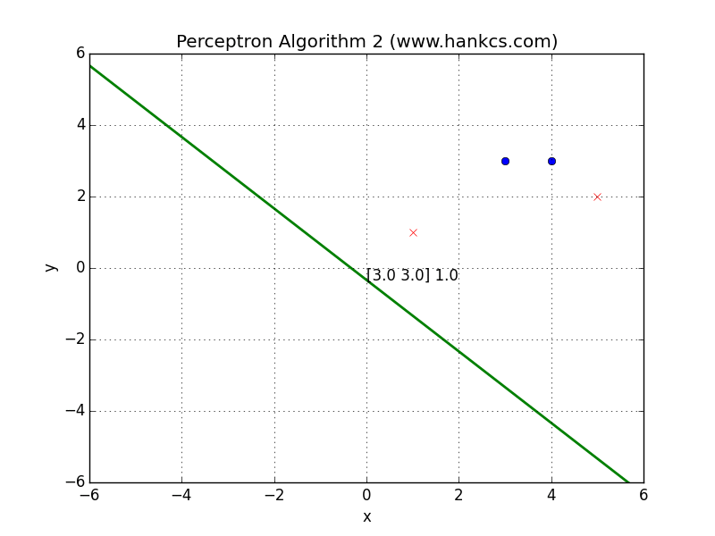
可视化

与算法1的结果相同,我们也可以将数据集改一下:
- training_set = np.array([[[3, 3], 1], [[4, 3], 1], [[1, 1], -1], [[5, 2], -1]])
会得到一个复杂一些的结果:
读后感
通过最简单的模型,学习到ML中的常用概念和常见流程。