Datacamp 笔记&代码 Unsupervised Learning in Python 第三章 Decorrelating your data and dimension reduction

更多原始数据文档和JupyterNotebook
Github: https://github.com/JinnyR/Datacamp_DataScienceTrack_Python

Datacamp track: Data Scientist with Python - Course 23 (3)

Exercise

Correlated data in nature

You are given an array grains giving the width and length of samples of grain. You suspect that width and length will be correlated. To confirm this, make a scatter plot of width vs length and measure their Pearson correlation.

Instruction

• Import:
  • matplotlib.pyplot as plt.
  • pearsonr from scipy.stats.
• Assign column 0 of grains to width and column 1 of grains to length.
• Make a scatter plot with width on the x-axis and lengthon the y-axis.
• Use the pearsonr() function to calculate the Pearson correlation of width and length.

import pandas as pd

grains = pd.read_csv('https://s3.amazonaws.com/assets.datacamp.com/production/course_2141/datasets/seeds-width-vs-length.csv', header=None).values

# Perform the necessary imports
import matplotlib.pyplot as plt
from scipy.stats import pearsonr

# Assign the 0th column of grains: width
width = grains[:,0]

# Assign the 1st column of grains: length
length = grains[:,1]

# Scatter plot width vs length
plt.scatter(width, length)
plt.axis('equal')
plt.show()

# Calculate the Pearson correlation
correlation, pvalue = pearsonr(width, length)

# Display the correlation
print(correlation)

0.8604149377143467

Exercise

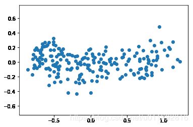
Decorrelating the grain measurements with PCA

You observed in the previous exercise that the width and length measurements of the grain are correlated. Now, you’ll use PCA to decorrelate these measurements, then plot the decorrelated points and measure their Pearson correlation.

Instruction

• Import PCA from sklearn.decomposition.
• Create an instance of PCA called model.
• Use the .fit_transform() method of model to apply the PCA transformation to grains. Assign the result to pca_features.
• The subsequent code to extract, plot, and compute the Pearson correlation of the first two columns pca_features has been written for you, so hit ‘Submit Answer’ to see the result!

# Import PCA
from sklearn.decomposition import PCA

# Create PCA instance: model
model = PCA()

# Apply the fit_transform method of model to grains: pca_features
pca_features = model.fit_transform(grains)

# Assign 0th column of pca_features: xs
xs = pca_features[:,0]

# Assign 1st column of pca_features: ys
ys = pca_features[:,1]

# Scatter plot xs vs ys
plt.scatter(xs, ys)
plt.axis('equal')
plt.show()

# Calculate the Pearson correlation of xs and ys
correlation, pvalue = pearsonr(xs, ys)

# Display the correlation
print(correlation)

7.474656899453042e-17

Exercise

The first principal component

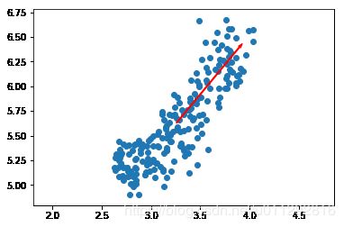
The first principal component of the data is the direction in which the data varies the most. In this exercise, your job is to use PCA to find the first principal component of the length and width measurements of the grain samples, and represent it as an arrow on the scatter plot.

The array grains gives the length and width of the grain samples. PyPlot (plt) and PCA have already been imported for you.

Instruction

• Make a scatter plot of the grain measurements. This has been done for you.
• Create a PCA instance called model.
• Fit the model to the grains data.
• Extract the coordinates of the mean of the data using the .mean_ attribute of model.
• Get the first principal component of model using the .components_[0,:] attribute.
• Plot the first principal component as an arrow on the scatter plot, using the plt.arrow() function. You have to specify the first two arguments - mean[0] and mean[1].

# Make a scatter plot of the untransformed points
plt.scatter(grains[:,0], grains[:,1])

# Create a PCA instance: model
model = PCA()

# Fit model to points
model.fit(grains)

# Get the mean of the grain samples: mean
mean = model.mean_

# Get the first principal component: first_pc
first_pc = model.components_[0,:]

# Plot first_pc as an arrow, starting at mean
plt.arrow(mean[0], mean[1], first_pc[0], first_pc[1], color='red', width=0.01)

# Keep axes on same scale
plt.axis('equal')
plt.show()

Exercise

Variance of the PCA features

The fish dataset is 6-dimensional. But what is its intrinsicdimension? Make a plot of the variances of the PCA features to find out. As before, samples is a 2D array, where each row represents a fish. You’ll need to standardize the features first.

Instruction

• Create an instance of StandardScaler called scaler.
• Create a PCA instance called pca.
• Use the make_pipeline() function to create a pipeline chaining scaler and pca.
• Use the .fit() method of pipeline to fit it to the fish samples samples.
• Extract the number of components used using the .n_components_ attribute of pca. Place this inside a range() function and store the result as features.
• Use the plt.bar() function to plot the explained variances, with features on the x-axis and pca.explained_variance_ on the y-axis.

import pandas as pd

df = pd.read_csv('https://s3.amazonaws.com/assets.datacamp.com/production/course_2234/datasets/fish.csv', header=None)
samples = df[list(range(1, len(df.columns)))].values # first column is the classes

# Perform the necessary imports
from sklearn.decomposition import PCA
from sklearn.preprocessing import StandardScaler
from sklearn.pipeline import make_pipeline
import matplotlib.pyplot as plt

# Create scaler: scaler
scaler = StandardScaler()

# Create a PCA instance: pca
pca = PCA()

# Create pipeline: pipeline
pipeline = make_pipeline(scaler, pca)

# Fit the pipeline to 'samples'
pipeline.fit(samples)

# Plot the explained variances
features = range(pca.n_components_)
plt.bar(features, pca.explained_variance_)
plt.xlabel('PCA feature')
plt.ylabel('variance')
plt.xticks(features)
plt.show()

Exercise

Dimension reduction of the fish measurements

In a previous exercise, you saw that 2 was a reasonable choice for the “intrinsic dimension” of the fish measurements. Now use PCA for dimensionality reduction of the fish measurements, retaining only the 2 most important components.

The fish measurements have already been scaled for you, and are available as scaled_samples.

Instruction

• Import PCA from sklearn.decomposition.
• Create a PCA instance called pca with n_components=2.
• Use the .fit() method of pca to fit it to the scaled fish measurements scaled_samples.
• Use the .transform() method of pca to transform the scaled_samples. Assign the result to pca_features.

from sklearn.preprocessing import StandardScaler
import pandas as pd

df = pd.read_csv('https://s3.amazonaws.com/assets.datacamp.com/production/course_2234/datasets/fish.csv', header=None)
features = df[list(range(1, len(df.columns)))] # first column is the classes

scaler = StandardScaler()
scaler.fit(features.values)
scaled_samples = scaler.transform(features.values)

# Import PCA
from sklearn.decomposition import PCA

# Create a PCA model with 2 components: pca
pca = PCA(n_components=2)

# Fit the PCA instance to the scaled samples
pca.fit(scaled_samples)

# Transform the scaled samples: pca_features
pca_features = pca.transform(scaled_samples)

# Print the shape of pca_features
print(pca_features.shape)

(85, 2)

Exercise

A tf-idf word-frequency array

In this exercise, you’ll create a tf-idf word frequency array for a toy collection of documents. For this, use the TfidfVectorizer from sklearn. It transforms a list of documents into a word frequency array, which it outputs as a csr_matrix. It has fit() and transform() methods like other sklearn objects.

You are given a list documents of toy documents about pets. Its contents have been printed in the IPython Shell.

Instruction

• Import TfidfVectorizer from sklearn.feature_extraction.text.
• Create a TfidfVectorizer instance called tfidf.
• Apply .fit_transform() method of tfidf to documents and assign the result to csr_mat. This is a word-frequency array in csr_matrix format.
• Inspect csr_mat by calling its .toarray() method and printing the result. This has been done for you.
• The columns of the array correspond to words. Get the list of words by calling the .get_feature_names() method of tfidf, and assign the result to words.

documents = ['cats say meow','dogs say woof', 'dogs chase cat']
print(documents)
             

['cats say meow', 'dogs say woof', 'dogs chase cat']

# Import TfidfVectorizer
from sklearn.feature_extraction.text import TfidfVectorizer

# Create a TfidfVectorizer: tfidf
tfidf = TfidfVectorizer() 

# Apply fit_transform to document: csr_mat
csr_mat = tfidf.fit_transform(documents)

# Print result of toarray() method
print(csr_mat.toarray())

# Get the words: words
words = tfidf.get_feature_names()

# Print words
print(words)

[[0.         0.62276601 0.         0.         0.62276601 0.4736296
  0.        ]
 [0.         0.         0.         0.51785612 0.         0.51785612
  0.68091856]
 [0.62276601 0.         0.62276601 0.4736296  0.         0.
  0.        ]]
['cat', 'cats', 'chase', 'dogs', 'meow', 'say', 'woof']

Exercise

Clustering Wikipedia part I

You saw in the video that TruncatedSVD is able to perform PCA on sparse arrays in csr_matrix format, such as word-frequency arrays. Combine your knowledge of TruncatedSVD and k-means to cluster some popular pages from Wikipedia. In this exercise, build the pipeline. In the next exercise, you’ll apply it to the word-frequency array of some Wikipedia articles.

Create a Pipeline object consisting of a TruncatedSVD followed by KMeans. (This time, we’ve precomputed the word-frequency matrix for you, so there’s no need for a TfidfVectorizer).

The Wikipedia dataset you will be working with was obtained from here.

Instruction

• Import:
  • TruncatedSVD from sklearn.decomposition.
  • KMeans from sklearn.cluster.
  • make_pipeline from sklearn.pipeline.
• Create a TruncatedSVD instance called svd with n_components=50.
• Create a KMeans instance called kmeans with n_clusters=6.
• Create a pipeline called pipeline consisting of svd and kmeans.

# Perform the necessary imports
from sklearn.decomposition import TruncatedSVD
from sklearn.cluster import KMeans
from sklearn.pipeline import make_pipeline

# Create a TruncatedSVD instance: svd
svd = TruncatedSVD(n_components=50)

# Create a KMeans instance: kmeans
kmeans = KMeans(n_clusters=6)

# Create a pipeline: pipeline
pipeline = make_pipeline(svd, kmeans)

Exercise

Clustering Wikipedia part II

It is now time to put your pipeline from the previous exercise to work! You are given an array articles of tf-idf word-frequencies of some popular Wikipedia articles, and a list titles of their titles. Use your pipeline to cluster the Wikipedia articles.

A solution to the previous exercise has been pre-loaded for you, so a Pipeline pipeline chaining TruncatedSVD with KMeans is available.

Instruction

• Import pandas as pd.
• Fit the pipeline to the word-frequency array articles.
• Predict the cluster labels.
• Align the cluster labels with the list titles of article titles by creating a DataFrame df with labels and titles as columns. This has been done for you.
• Use the .sort_values() method of df to sort the DataFrame by the 'label' column, and print the result.
• Hit ‘Submit Answer’ and take a moment to investigate your amazing clustering of Wikipedia pages!

import pandas as secret_pandas # since the import is part of the exercise!
from scipy.sparse import csr_matrix

df = secret_pandas.read_csv('https://s3.amazonaws.com/assets.datacamp.com/production/course_2141/datasets/wikipedia-vectors.csv', index_col=0)
articles = csr_matrix(df.transpose())
titles = list(df.columns)

# a model solution to previous exercise
from sklearn.decomposition import TruncatedSVD
from sklearn.cluster import KMeans
from sklearn.pipeline import make_pipeline

svd = TruncatedSVD(n_components=50)
kmeans = KMeans(n_clusters=6)
pipeline = make_pipeline(svd, kmeans)

# Import pandas
import pandas as pd

# Fit the pipeline to articles
pipeline.fit(articles)

# Calculate the cluster labels: labels
labels = pipeline.predict(articles)

# Create a DataFrame aligning labels and titles: df
df = pd.DataFrame({'label': labels, 'article': titles})

# Display df sorted by cluster label
print(df.sort_values('label'))

    label                                        article
29      0                               Jennifer Aniston
27      0                                 Dakota Fanning
26      0                                     Mila Kunis
25      0                                  Russell Crowe
24      0                                   Jessica Biel
23      0                           Catherine Zeta-Jones
22      0                              Denzel Washington
21      0                             Michael Fassbender
20      0                                 Angelina Jolie
28      0                                  Anne Hathaway
19      1  2007 United Nations Climate Change Conference
18      1  2010 United Nations Climate Change Conference
17      1  Greenhouse gas emissions by the United States
16      1                                        350.org
15      1                                 Kyoto Protocol
14      1                                 Climate change
12      1                                   Nigel Lawson
11      1       Nationally Appropriate Mitigation Action
10      1                                 Global warming
13      1                               Connie Hedegaard
41      2                                    Hepatitis B
42      2                                    Doxycycline
43      2                                       Leukemia
44      2                                           Gout
45      2                                    Hepatitis C
46      2                                     Prednisone
47      2                                          Fever
48      2                                     Gabapentin
49      2                                       Lymphoma
40      2                                    Tonsillitis
0       2                                       HTTP 404
5       2                                         Tumblr
1       2                                 Alexa Internet
2       2                              Internet Explorer
3       2                                    HTTP cookie
4       2                                  Google Search
6       2                    Hypertext Transfer Protocol
7       2                                  Social search
8       2                                        Firefox
9       2                                       LinkedIn
58      3                                         Sepsis
30      4                  France national football team
31      4                              Cristiano Ronaldo
38      4                                         Neymar
37      4                                       Football
36      4              2014 FIFA World Cup qualification
35      4                Colombia national football team
34      4                             Zlatan Ibrahimović
33      4                                 Radamel Falcao
32      4                                   Arsenal F.C.
39      4                                  Franck Ribéry
57      5                          Red Hot Chili Peppers
56      5                                       Skrillex
55      5                                  Black Sabbath
51      5                                     Nate Ruess
53      5                                   Stevie Nicks
52      5                                     The Wanted
50      5                                   Chad Kroeger
54      5                                 Arctic Monkeys
59      5                                    Adam Levine