数据分析学习总结笔记17：文本分析入门案例实战

1 数据准备

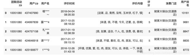
数据样例如下， 数据总量为7.7万+：

本节通过一个实战的例子来展示文本分析的最简单流程。首先设定因变量为原始数据中的"评分"。自变量是"评价内容"，这里根据评价内容提取TF-IDF特征。之后，通过评价内容的特征建模预测下整体评分。

import jieba #导入分词模块
import pandas as pd # 导入Pandas模块

# 1. 导入数据
comments_df = pd.read_excel("https://github.com/xiangyuchang/xiangyuchang.github.io/blob/master/BearData/comment_nm.xlsx?raw=true") #读入数据
print('数据的维度是：', comments_df.shape)
comments_df.head() #查看数据的前5行

# 2. 清洗数据, 删除空的数据
def clean_sents(txt):
    txt = str(txt) if txt is not None else ""
    if len(txt) == 0:
        return None
    else:
        return txt
        
comments_df2["评价内容"] = comments_df2["评价内容"].apply(clean_sents)
comments_df2 = comments_df2[comments_df2["评价内容"] != "nan"]
len(comments_df2)

# 运行结果
# 58117

以上只是最基本的数据清洗(删除缺失值)， 这里不再赘述。过滤后， 样本量为5.8W+条， 减少2.2万+。

2 分词

文本分析的第一步是分词。常用中文包是jieba: https://github.com/fxsjy/jieba.

再次声明， 本书为平滑学习曲线， 仅对最重要的函数进行调用和说明， 在实际中不够用时请自行翻阅对应的官方文档。成熟的开源库基本都有完善的文档， 即学即用即可。

# 引入停用词文本，请在如下网址下载：https://github.com/zhiyiZeng/cluebearpython/blob/master/chapter8/data/stopwords.txt

stopwords_file = "stopwords.txt"
with open(os.path.join(path, stopwords_file), "r", encoding="utf8") as f:
    stopwords_list = [word.strip() for word in f.read()]

def filter_stopwords(txt):
    """过滤停用词"""
    sent = jieba.lcut(txt)
    words = []
    for word in sent:
        if(word in stopwords_list):
            continue
        else:
            words.append(word)
    return words
    
comments_df2["评价内容"] = comments_df2["评价容"].apply(filter_stopwords)
comments_df2.head()

本例代码先导入停用词库， 再用Pandas的apply()方法对每条评论进行分词， 分词完成后对每个单词判断是否在停用词库中， 如果存在则过滤。最终再返回过滤后的分词结果。最终结果如下。

3 统计词频

在提取feature之前， 推荐先画个词云， 也是探索性分析的一部分， 以便对数据整体有个印象。

# 3. 切分训练集和验证集和测试集
from sklearn.model_selection import train_test_split

train_X, val_X, train_y, val_y = train_test_split(comments_df2["评价内容"], comments_df2["评分"], test_size=0.3)

val_X, test_X, val_y, test_y = train_test_split(val_X, val_y, test_size=0.5)

# 4. 统计词频
from nltk import FreqDist

# 把所有词和对应的词频放在一个list里
all_words = []

for comment in comments_df2["评价内容"]:
    all_words.extend(comment)

len(all_words)

fdisk = FreqDist(all_words)

TOP_COMMON_WORDS = 1000

most_common_words = fdisk.most_common(TOP_COMMON_WORDS)


most_common_words[:10]

最终结果， 只截取前10条数据， 第一列为词， 第二列为对应词频。

4 词云

词云， 即把词展现在有一定形状的图片上。同时， 按照词的词频大小， 生成不同尺寸的词。这样， 就能够非常直观的区分出不同词的词频大小关系。

注意， 词云是对于文本类型数据的探索性分析，且仅仅是为了能够直观反映词频大小关系， 而非精确度量。因此， 不应将词云的结果完全作为分析的依据， 但是词云仍然有很高探索性数据分析的价值。画词云的工具， 推荐wordcloud（https://github.com/amueller/word_cloud）。

from wordcloud import WordCloud
import matplotlib.pyplot as plt
from PIL import Image
import numpy as np

# 词云形状
mask = np.array(Image.open(os.path.join(path, "火锅图片.png")))
wc = WordCloud(font_path=os.path.join(path, "simkai.ttf"),
               background_color="white",
               contour_width=3,
               contour_color='steelblue',
               mask=mask,
               width=1000,
               height=1000)
wc.generate_from_frequencies(dict(most_common_words))
fig = plt.figure(figsize=(10, 10))
plt.imshow(wc)

# 取消坐标轴
plt.axis("off")

# 保存图片
plt.savefig(os.path.join(path, "火锅词云.png"), dpi=1000)

# 展示图片
plt.show()

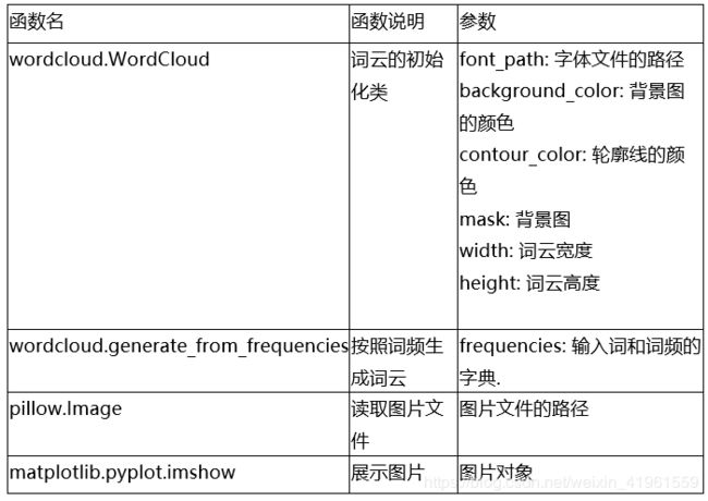
这段代码的逻辑是：先初始化WordCloud类， 这里定义词云的一些基本配置， 再对实例化的对象输入词频字典。最终用matplotlib展示图片并保存即可。

注意：

1. 这里的PIL包是指pillow， 安装的时候仍然为pip install pillow， 但引入的时候包名PIL， 这是因为旧版的pillow已经不再被官方维护， 后来另有开发者进行重新维护， 为了区分， 才导致这一情况。使用时记得这一小变化即可。
   2.plt.savefig()一定要在plt.show()之前， 否则会保存为空图片， 这是因为plt.show()会对清空画布中的对象。

最终运行结果：

5 提取特征

下面进行最关键的一步，即提起TF-IDF特征。

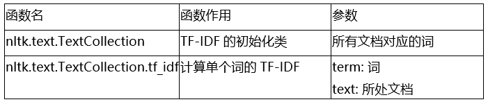
from nltk.text import TextCollection

tfidf_generator = TextCollection(train_X.values.tolist())

def extract_tfidf(texts, targets, text_collection, common_words):
    """
    提取文本的tf-idf.
        texts: 输入的文本.
        targets: 对应的评价.
        text_collection: 预先初始化的TextCollection.
        common_words: 输入的前N个词作为特征进行计算.
    """
    # 得到行向量的维度
    n_sample = len(texts)
    # 得到列向量的维度
    n_feat = len(common_words)
    # 初始化X矩阵, X为最后要输出的TF-IDF矩阵
    X = np.zeros([n_sample, n_feat])
    y = np.zeros(n_sample) 
    for i, text in enumerate(texts):
        if i % 5000 == 0:
            print("已经完成{}个样本的特征提取.".format(i))
        # 每一行对应一个文档, 计算这个文档中的词的tf-idf, 没出现的词则为0
        feature_vector = []
        for word in common_words:
            if word in text:
                tf_idf = text_collection.tf_idf(word, text)
            else:
                tf_idf = 0.0
            feature_vector.append(tf_idf)           
        X[i, :] = np.array(feature_vector)
        y[i] = targets.iloc[i]      
    return X, y

cleaned_train_X, cleaned_train_y = extract_tfidf(train_X, train_y, tfidf_generator, dict(most_common_words).keys())
cleaned_val_X, cleaned_val_y = extract_tfidf(val_X, val_y, tfidf_generator, dict(most_common_words).keys())

上述代码逻辑为：分别将需要处理的训练集和验证集的X所对应的每一行(即每一个文档)， 匹配总词数， 计算得到每一行的每一个词的tf-idf， 最后输出。

6 用sklearn进行训练

最后， 将提取的TF-IDF扔到模型进行训练即可。需要什么模型视具体需求而定, 这里不再展开，读者可自行尝试。下面的例子，展示了使用SVM进行训练的代码。

from sklearn import svm

clf = svm.SVC()
clf.fit(cleaned_train_X, cleaned_train_y)
clf.score(cleaned_train_X, cleaned_train_y)
clf.score(cleaned_val_X, cleaned_val_y)

若需进一步了解更多文本探索性分析（词性分析、情感分析等）可查看：数据分析学习总结笔记16：NLP自然语言处理与文本探索性分析

本文主要参考于：
Python数据科学实践 | 文本分析2

相关笔记：

1. Python相关实用技巧01：安装Python库超实用方法，轻松告别失败！
2. Python相关实用技巧02：Python2和Python3的区别
3. Python相关实用技巧03：14个对数据科学最有用的Python库
4. Python相关实用技巧04：网络爬虫之Scrapy框架及案例分析
5. Python相关实用技巧05：yield关键字的使用
6. Scrapy爬虫小技巧01：轻松获取cookies
7. Scrapy爬虫小技巧02：HTTP status code is not handled or not allowed的解决方法
8. 数据分析学习总结笔记01：情感分析
9. 数据分析学习总结笔记02：聚类分析及其R语言实现
10. 数据分析学习总结笔记03：数据降维经典方法
11. 数据分析学习总结笔记04：异常值处理
12. 数据分析学习总结笔记05：缺失值分析及处理
13. 数据分析学习总结笔记06：T检验的原理和步骤
14. 数据分析学习总结笔记07：方差分析
15. 数据分析学习总结笔记07：回归分析概述
16. 数据分析学习总结笔记08：数据分类典型方法及其R语言实现
17. 数据分析学习总结笔记09：文本分析
18. 数据分析学习总结笔记10：网络分析
19. 数据分析学习总结笔记11：空间复杂度和时间复杂度
20. 数据分析学习总结笔记12：空间自相关——空间位置与相近位置的指标测度
21. 数据分析学习总结笔记13：生存分析及Python实现
22. 数据分析学习总结笔记14：A/B Test及Python实现
23. 数据分析学习总结笔记15：时间序列分析及Python实现
24. 数据分析学习总结笔记16：NLP自然语言处理与文本探索性分析
25. 笔记专栏——数据研发笔试Leetcode刷题