深度模型训练之learning rate

下文根据Tensorflow中learning rate decay的奇技淫巧整理，增加了相关源码，另外针对不同方法，不同特点，在后续会给出更多的实例化。
深度学习中参数更新的方法想必大家都十分清楚了——sgd，adam等等，孰优孰劣相关的讨论也十分广泛。可是，learning rate的衰减策略大家有特别关注过吗？
说实话，以前我也只使用过指数型和阶梯型的下降法，并不认为它对深度学习调参有多大帮助。但是，最近的学习和工作中逐渐接触到了各种奇形怪状的lr策略，可以说大大刷新了三观，在此也和大家分享一下学习经验。
learning rate衰减策略文件在tensorflow/tensorflow/python/training/learning_rate_decay.py中，函数中调用方法类似tf.train.exponential_decay就可以了。
以下，我将在ipython中逐个介绍各种lr衰减策略。本文的示例代码可以再我的github上找到：参考链接

1.基于指数型的衰减

下面的几个实现都是基于指数型的衰减。个人理解其问题在于一开始lr就快速下降，在复杂问题中可能会导致快速收敛于局部最小值而没有较好地探索一定范围内的参数空间。

1.1.exponential_decay

让学习率满足一些性质的情况下不断下降，这里指数衰减的一个性质是它的衰减值是当前值的一部分，也就是说$\frac{dN}{dt}=-\lambda N$，其中N是要进行衰减的值，例如学习率。 为了满足上面的性质，具体的衰减如下，$N(t)=N_0{e}^{-\lambda t}$,

计算公式
$$decayed\_learning\_rate=learning\_rate\ast decay\_rat{e}^{global\_step/decay\_steps}$$

函数原型
exponential_decay(learning_rate, global_step, decay_steps, decay_rate, staircase=False, name=None)

• learning_rate：初始学习率．
• global_step：用于衰减计算的全局步数，非负。用于逐步计算衰减指数。
• decay_steps：衰减步数，必须是正值．决定衰减周期．
• decay_rate：衰减率．
• staircase：若为True，则以不连续的间隔衰减学习速率即阶梯型衰减（就是在一段时间内或相同的epoch_{（往往是相同的epoch内）}内保持相同的学习率）；若为False，则是标准指数型衰减．
• name：操作的名称，默认为ExponentialDecay．（可选项）

指数型lr衰减法是最常用的衰减方法，在大量模型中都广泛使用。

特点
简单直接，收敛速度快．

代码示例

import matplotlib.pyplot as plt
import tensorflow as tf
#global_step = tf.Variable(0, name='global_step', trainable=False)

y = []
z = []
N = 200
with tf.Session() as sess:
    sess.run(tf.global_variables_initializer())
    for global_step in range(N):
        # 阶梯型衰减
        learing_rate1 = tf.train.exponential_decay(
            learning_rate=0.5, global_step=global_step, decay_steps=10, decay_rate=0.9, staircase=True)
        # 标准指数型衰减
        learing_rate2 = tf.train.exponential_decay(
            learning_rate=0.5, global_step=global_step, decay_steps=10, decay_rate=0.9, staircase=False)
        lr1 = sess.run([learing_rate1])
        lr2 = sess.run([learing_rate2])
        y.append(lr1[0])
        z.append(lr2[0])

x = range(N)
fig = plt.figure()
ax = fig.add_subplot(111)
ax.set_ylim([0, 0.55])
plt.plot(x, y, 'r-', linewidth=2)
plt.plot(x, z, 'g-', linewidth=2)
plt.title('exponential_decay')
ax.set_xlabel('step')
ax.set_ylabel('learing rate')
plt.show()

效果图

红色为阶梯型衰减，绿色为标准指数衰减

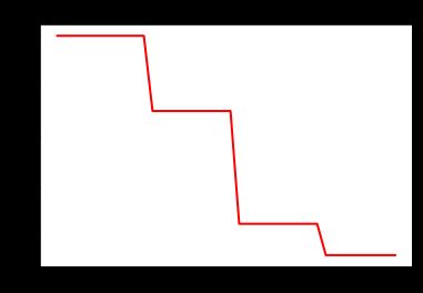
1.2.piecewise_constant

分段常数衰减就是在定义好的区间上，分别设置不同的常数值，作为学习率的初始值和后续衰减的取值．

函数原型

piecewise_constant(x, boundaries, values, name=None)

• x：0-D标量Tensor．
• boundaries：边界，tensor或list.
• values：指定定义区间的值．
• name：操作的名称，默认为PiecewiseConstant．

分段常数下降法类似于exponential_decay中的阶梯式下降法，不过各阶段的值是自己设定的。

其中，x即为global step，boundaries=[step_1, step_2, …, step_n]定义了在第几步进行lr衰减，values=[val_0, val_1, val_2, …, val_n]定义了lr的初始值和后续衰减时的具体取值。需要注意的是，values应该比boundaries长一个维度。

特点
这种方法有助于使用者针对不同任务进行精细地调参，在任意步长后下降任意数值的learning rate。

代码示例

# piecewise_constant 阶梯式下降法
import matplotlib.pyplot as plt
import tensorflow as tf

#global_step = tf.Variable(0, name='global_step', trainable=False)
boundaries = [10, 20, 30]
learing_rates = [0.1, 0.07, 0.025, 0.0125]
y = []
N = 40
with tf.Session() as sess:
    sess.run(tf.global_variables_initializer())
    for global_step in range(N):
        learing_rate = tf.train.piecewise_constant(global_step, boundaries=boundaries, values=learing_rates)
        lr = sess.run([learing_rate])
        y.append(lr[0])

x = range(N)
plt.plot(x, y, 'r-', linewidth=2)
plt.title('piecewise_constant')
plt.show()

1.3.polynomial_decay

函数使用多项式衰减，以给定的decay_steps将初始学习率（learning_rate）衰减至指定的学习率（end_learning_rate）．

计算方法
$$global\_step=min(global\_step,decay\_steps)$$
$$decayed\_learnin{g}_{r}ate=(learning\_rate-end\_learning\_rate)\ast (1-global\_step/decay\_steps{)}^{power}+en{d}_{l}earnin{g}_{r}ate$$

函数原型

polynomial_decay(learning_rate, global_step, decay_steps, end_learning_rate=0.0001, power=1.0, cycle=False, name=None)

• learning_rate：初始学习率．
• global_step：用于衰减计算的全局步数，非负.
• decay_steps：衰减步数，必须是正值．
• end_learning_rate：最低的最终学习率．
• power：多项式的幂，默认为1.0（线性）．
• cycle：学习率下降后是否重新上升．参数cycle决定学习率是否在下降后重新上升．若cycle为True，则学习率下降后重新上升；使用decay_steps的倍数，取第一个大于global_steps的结果．
• name：操作的名称，默认为PolynomialDecay。

参数cycle目的：防止神经网络训练后期学习率过小导致网络一直在某个局部最小值中振荡；这样，通过增大学习率可以跳出局部极小值．

示例代码

# 学习率下降后是否重新上升
import matplotlib.pyplot as plt
import tensorflow as tf
y = []
z = []
N = 200
#global_step = tf.Variable(0, name='global_step', trainable=False)

with tf.Session() as sess:
    sess.run(tf.global_variables_initializer())
    for global_step in range(N):
        # cycle=False
        learing_rate1 = tf.train.polynomial_decay(
            learning_rate=0.1, global_step=global_step, decay_steps=50,
            end_learning_rate=0.01, power=0.5, cycle=False)
        # cycle=True
        learing_rate2 = tf.train.polynomial_decay(
            learning_rate=0.1, global_step=global_step, decay_steps=50,
            end_learning_rate=0.01, power=0.5, cycle=True)
        lr1 = sess.run([learing_rate1])
        lr2 = sess.run([learing_rate2])
        y.append(lr1[0])
        z.append(lr2[0])

x = range(N)
fig = plt.figure()
ax = fig.add_subplot(111)
plt.plot(x, z, 'g-', linewidth=2)
plt.plot(x, y, 'r--', linewidth=2)
plt.title('polynomial_decay')
ax.set_xlabel('step')
ax.set_ylabel('learing rate')
plt.show()

运行结果

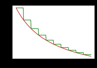
1.4.natural_exp_decay

应用自然指数衰减的学习率．
natural_exp_decay 和 exponential_decay 形式近似，natural_exp_decay的底数是e．

计算方法
$$decayed\_learning\_rate=learning\_rate\ast exp(-decay\_rate\ast global\_step)$$

函数原型

natural_exp_decay(learning_rate, global_step, decay_steps, decay_rate, staircase=False, name=None)

• learning_rate：初始学习率．
• global_step：用于衰减计算的全局步数，非负.
• decay_steps：衰减步数．
• decay_rate：衰减率．
• staircase：若为True，则是离散的阶梯型衰减（就是在一段时间内或相同的eproch内保持相同的学习率）；若为False，则是标准型衰减．
• name: 操作的名称，默认为ExponentialTimeDecay．

特点
自然指数衰减比指数衰减要快的多，一般用于较快收敛，容易训练的网络．

示例代码

import matplotlib.pyplot as plt
import tensorflow as tf
#global_step = tf.Variable(0, name='global_step', trainable=False)

y = []
z = []
w = []
N = 200
with tf.Session() as sess:
    sess.run(tf.global_variables_initializer())
    for global_step in range(N):
        # 阶梯型衰减
        learing_rate1 = tf.train.natural_exp_decay(
            learning_rate=0.5, global_step=global_step, decay_steps=10, decay_rate=0.9, staircase=True)
        # 标准指数型衰减
        learing_rate2 = tf.train.natural_exp_decay(
            learning_rate=0.5, global_step=global_step, decay_steps=10, decay_rate=0.9, staircase=False)
        # 指数衰减
        learing_rate3 = tf.train.exponential_decay(
            learning_rate=0.5, global_step=global_step, decay_steps=10, decay_rate=0.9, staircase=False)
        lr1 = sess.run([learing_rate1])
        lr2 = sess.run([learing_rate2])
        lr3 = sess.run([learing_rate3])
        y.append(lr1[0])
        z.append(lr2[0])
        w.append(lr3[0])

x = range(N)
fig = plt.figure()
ax = fig.add_subplot(111)
ax.set_ylim([0, 0.55])
plt.plot(x, y, 'r-', linewidth=2)
plt.plot(x, z, 'g-', linewidth=2)
plt.plot(x, w, 'b-', linewidth=2)
plt.title('natural_exp_decay')
ax.set_xlabel('step')
ax.set_ylabel('learing rate')
plt.show()

运行结果

1.5.inverse_time_decay

该函数应用反向衰减函数提供初始学习速率．利用global_step来计算衰减的学习速率．

计算方法

staircase为False:
$$decayed\_learning\_rate=learning\_rate/(1+decay\_rate\ast global\_step/decay\_step)$$
staircase为True
$$decayed\_learnin{g}_{r}ate=learning\_rate/(1+decay\_rate\ast floor(globa{l}_{s}tep/deca{y}_{s}tep))$$
函数原型

inverse_time_decay(learning_rate, global_step, decay_steps, decay_rate, staircase=False, name=None)

• learning_rate：初始学习率．
• global_step：用于衰减计算的全局步数．
• decay_steps：衰减步数．
• decay_rate：衰减率．
• staircase：是否应用离散阶梯型衰减．（否则为连续型）
• name：操作的名称，默认为InverseTimeDecay．

import matplotlib.pyplot as plt
import tensorflow as tf
y = []
z = []
N = 200
#global_step = tf.Variable(0, name='global_step', trainable=False)

with tf.Session() as sess:
    sess.run(tf.global_variables_initializer())
    for global_step in range(N):
        # 阶梯型衰减
        learing_rate1 = tf.train.inverse_time_decay(
            learning_rate=0.1, global_step=global_step, decay_steps=20,
            decay_rate=0.2, staircase=True)
        # 连续型衰减
        learing_rate2 = tf.train.inverse_time_decay(
            learning_rate=0.1, global_step=global_step, decay_steps=20,
            decay_rate=0.2, staircase=False)
        lr1 = sess.run([learing_rate1])
        lr2 = sess.run([learing_rate2])

        y.append(lr1[0])
        z.append(lr2[0])

x = range(N)
fig = plt.figure()
ax = fig.add_subplot(111)
plt.plot(x, z, 'r-', linewidth=2)
plt.plot(x, y, 'g-', linewidth=2)
plt.title('inverse_time_decay')
ax.set_xlabel('step')
ax.set_ylabel('learing rate')
plt.show()

运行结果

2.基于余弦的衰减

下面的几个实现，都是基于cos函数的。

2.1.cosine_decay

cosine_decay是近一年才提出的一种lr衰减策略，基本形状是余弦函数。其方法是基于论文实现的：
SGDR: Stochastic Gradient Descent with Warm Restarts

计算方法

global_step = min(global_step, decay_steps)
cosine_decay = 0.5 * (1 + cos(pi * global_step / decay_steps))
decayed = (1 - alpha) * cosine_decay + alpha
decayed_learning_rate = learning_rate * decayed

函数原型
cosine_decay(learning_rate, global_step, decay_steps, alpha=0.0, name=None)

• learning_rate：标初始学习率．
• global_step：用于衰减计算的全局步数.
• decay_steps：衰减步数．
• alpha：最小学习率（learning_rate的部分）。
• name：操作的名称，默认为CosineDecay

import matplotlib.pyplot as plt
import tensorflow as tf
y = []
z = []
N = 200
#global_step = tf.Variable(0, name='global_step', trainable=False)

with tf.Session() as sess:
    sess.run(tf.global_variables_initializer())
    for global_step in range(N):
        # 阶梯型衰减
        learing_rate1 = tf.train.cosine_decay(
            learning_rate=0.1, global_step=global_step, decay_steps=150,
            alpha=0.0)
        # 连续型衰减
        learing_rate2 = tf.train.cosine_decay(
            learning_rate=0.1, global_step=global_step, decay_steps=150,
            alpha=0.3)
        lr1 = sess.run([learing_rate1])
        lr2 = sess.run([learing_rate2])

        y.append(lr1[0])
        z.append(lr2[0])

x = range(N)
fig = plt.figure()
ax = fig.add_subplot(111)
plt.plot(x, z, 'r-', linewidth=2)
plt.plot(x, y, 'g-', linewidth=2)
plt.title('cosine_decay')
ax.set_xlabel('step')
ax.set_ylabel('learing rate')
plt.show()

运行效果

2.2.cosine_decay_restarts

cosine_decay_restarts是cosine_decay的cycle版本。first_decay_steps是指第一次完全下降的step数，t_mul是指每一次循环的步数都将乘以t_mul倍，m_mul指每一次循环重新开始时的初始lr是上一次循环初始值的m_mul倍。

函数原型
cosine_decay_restarts(learning_rate, global_step, first_decay_steps, t_mul=2.0, m_mul=1.0, alpha=0.0, name=None)

• learning_rate ：标量float32或float64 Tensor或Python数字。 初始学习率。
• global_step ：标量int32或int64 Tensor或Python数字。 用于衰减计算的全局步骤。
• first_decay_steps ：标量int32或int64 Tensor或Python数字。 衰减的步骤数。
• t_mul ：标量float32或float64 Tensor或Python数字。 用于导出第i个周期中的迭代次数
• m_mul ：标量float32或float64 Tensor或Python数字。 用于导出第i个周期的初始学习率：
• alpha ：标量float32或float64 Tensor或Python数字。 最小学习率值作为learning_rate的一部分。
• name ：String。 操作的可选名称。 默认为’SGDRDecay’。

特点
余弦函数式的下降模拟了大lr找潜力区域然后小lr快速收敛的过程，加之restart带来的cycle效果，有涨1-2个点的可能。

示例代码

 import matplotlib.pyplot as plt
import tensorflow as tf
y = []
z = []
N = 1000
#global_step = tf.Variable(0, name='global_step', trainable=False)

with tf.Session() as sess:
    sess.run(tf.global_variables_initializer())
    for global_step in range(N):
        # 阶梯型衰减
        learing_rate1 = tf.train.cosine_decay_restarts(
            learning_rate=0.1, global_step=global_step,t_mul=2.0,m_mul=0.5, alpha=0.0, first_decay_steps=200)
        # 连续型衰减
        learing_rate2 = tf.train.cosine_decay_restarts(
            learning_rate=0.1, global_step=global_step, t_mul=2.0,m_mul=1.0, alpha=0.0,first_decay_steps=200)
        lr1 = sess.run([learing_rate1])
        lr2 = sess.run([learing_rate2])

        y.append(lr1[0])
        z.append(lr2[0])

x = range(N)
fig = plt.figure()
ax = fig.add_subplot(111)
plt.plot(x, y, 'r-', linewidth=2)
plt.plot(x, z, 'g-', linewidth=2)
plt.title('cosine_decay_restarts')
ax.set_xlabel('step')
ax.set_ylabel('learing rate')
plt.show()

运行效果

红色线条t_mul=2.0，m_mul=0.5，蓝色线条t_mul=2.0，m_mul=1.0

2.3.linear_cosine_decay

linear_cosine_decay的参考文献是Neural Optimizer Search with Reinforcement Learning，主要应用领域是增强学习领域，本人未尝试过。可以看出，该方法也是基于余弦函数的衰减策略。

计算公式

global_step=min(global_step,decay_steps)
linear_decay=(decay_steps-global_step)/decay_steps)
cosine_decay = 0.5*(1+cos(pi*2*num_periods*global_step/decay_steps))
decayed=(alpha+linear_decay)*cosine_decay+beta
decayed_learning_rate=learning_rate*decayed

函数原型
linear_cosine_decay(learning_rate, global_step, decay_steps, num_periods=0.5, alpha=0.0, beta=0.001, name=None)

• learning_rate：标初始学习率．
• global_step：用于衰减计算的全局步数.
• decay_steps：衰减步数。
• num_periods：衰减余弦部分的周期数．
• alpha：见计算．
• beta：见计算．
• name：操作的名称，默认为LinearCosineDecay。

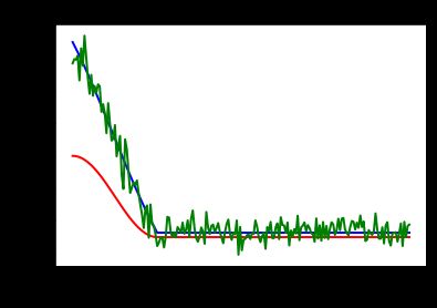
2.4.noisy_linear_cosine_decay

将噪声线性余弦衰减应用于学习率．
计算方法
与linear_cosine_decay相同

函数原型

• learning_rate：标初始学习率．
• global_step：用于衰减计算的全局步数.
• decay_steps：衰减步数．
• initial_variance：噪声的初始方差．
• variance_decay：衰减噪声的方差．
• num_periods：衰减余弦部分的周期数．
• alpha：见计算．
• beta：见计算．
• name：操作的名称，默认为NoisyLinearCosineDecay．

特点

根据论文Neural Optimizer Search with Reinforcement Learning提出．在衰减过程中加入了噪声，一定程度上增加了线性余弦衰减的随机性和可能性．

示例代码：

import matplotlib.pyplot as plt
import tensorflow as tf
y = []
z = []
w = []
N = 200
#global_step = tf.Variable(0, name='global_step', trainable=False)

with tf.Session() as sess:
    sess.run(tf.global_variables_initializer())
    for global_step in range(N):
        # 余弦衰减
        learing_rate1 = tf.train.cosine_decay(
            learning_rate=0.1, global_step=global_step, decay_steps=50,
            alpha=0.5)
        # 线性余弦衰减
        learing_rate2 = tf.train.linear_cosine_decay(
            learning_rate=0.1, global_step=global_step, decay_steps=50,
            num_periods=0.2, alpha=0.5, beta=0.2)
        # 噪声线性余弦衰减
        learing_rate3 = tf.train.noisy_linear_cosine_decay(
            learning_rate=0.1, global_step=global_step, decay_steps=50,
            initial_variance=0.01, variance_decay=0.1, num_periods=0.2, alpha=0.5, beta=0.2)
        lr1 = sess.run([learing_rate1])
        lr2 = sess.run([learing_rate2])
        lr3 = sess.run([learing_rate3])
        y.append(lr1[0])
        z.append(lr2[0])
        w.append(lr3[0])

x = range(N)
fig = plt.figure()
ax = fig.add_subplot(111)
plt.plot(x, y, 'r-', linewidth=2)
plt.plot(x, z, 'b-', linewidth=2)
plt.plot(x, w, 'g-', linewidth=2)
plt.title('cosine_decay')
ax.set_xlabel('step')
ax.set_ylabel('learing rate')
plt.show()

3.自定义

3.1.auto_learning_rate_decay

当然大家还可以自定义学习率衰减策略，如设置检测器监控valid的loss或accuracy值，若一定时间内loss持续有效下降／acc持续有效上升则保持lr，否则下降；loss上升／acc下降地越厉害，lr下降的速度就越快等等自适性方案。

4.小结

在我的实际使用中，最常用的就是exponential_decay，但是可以尝试一下cosine_decay_restarts，一定会带给你惊喜的~

参考文献

• Tensorflow中learning rate decay的奇技淫巧
• TensorFlow学习－－学习率衰减/learning rate decay