Jupyter练习
一、安装与使用
安装Ipython与Jupyter,安装好后,接着安装pandas、seaborn、statsmodels库。
或者直接安装anaconda,里面有Jupyter Notebook,直接启动,自动打开一个浏览器,创建一个新的Python3文件。
二、问题解答
导入数据分析要用到的各种库并且导入数据
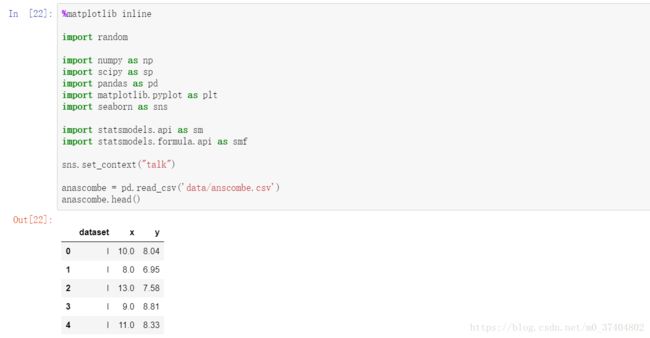
Part 1
For each of the four datasets...
- Compute the mean and variance of both x and y
- Compute the correlation coefficient between x and y
- Compute the linear regression line: y=β0+β1x+ϵ (hint: use statsmodels and look at the Statsmodels notebook)
(1)Compute the mean and variance of both x and y
gp = anascombe.groupby('dataset') #对数据集按照dataset列进行分组

#分别对四个类别的dataset输出x、y的均值和方差
for index in ['I','II',"III","IV"]:
    print("The " + index + " dataset:")
    mean_x = gp.get_group(index)['x'].mean()
    mean_y = gp.get_group(index)['y'].mean()
    var_x =  gp.get_group(index)['x'].var()
    var_y =  gp.get_group(index)['y'].var()
    print("  x的均值",mean_x)
    print("  y的均值", mean_y)
    print("  x的方差", var_x)
    print("  y的方差", var_y)
    print("")
output:
The I dataset:
  x的均值 9.0
  y的均值 7.500909090909093
  x的方差 11.0
  y的方差 4.127269090909091

The II dataset:
  x的均值 9.0
  y的均值 7.500909090909091
  x的方差 11.0
  y的方差 4.127629090909091

The III dataset:
  x的均值 9.0
  y的均值 7.500000000000001
  x的方差 11.0
  y的方差 4.12262

The IV dataset:
  x的均值 9.0
  y的均值 7.50090909090909
  x的方差 11.0
y的方差 4.12324909090909(2)Compute the correlation coefficient between x and y
cor_matrix = gp.corr() #求出相关系数矩阵
print("相关系数矩阵:")
print(cor_matrix)
print("")
#分别得出每个dataset的相关系数
for index in ['I','II',"III","IV"]:
    print("dataset " + index + " 相关系数 : ",cor_matrix['x'][index]['y'])
output:
相关系数矩阵:
                  x         y
dataset
I       x  1.000000  0.816421
        y  0.816421  1.000000
II      x  1.000000  0.816237
        y  0.816237  1.000000
III     x  1.000000  0.816287
        y  0.816287  1.000000
IV      x  1.000000  0.816521
        y  0.816521  1.000000

dataset I 相关系数 :  0.81642051634484
dataset II 相关系数 :  0.8162365060002428
dataset III 相关系数 :  0.8162867394895981
dataset IV 相关系数 :  0.8165214368885028
(3)Compute the linear regression line: y=β0+β1x+ϵ
for index in ['I','II','III','IV']:
    x1 = gp.get_group(index)['x']
    y1 = gp.get_group(index)['y']
    t = sm.add_constant(x1)
    stats_models = sm.OLS(y1,t)
    stats_models1 = stats_models.fit()
    print(stats_models1.summary())
    print("\n\n")
    print('we can see that params are:')
    print(stats_models1.params)
output:
   OLS Regression Results
==============================================================================
Dep. Variable:                      y   R-squared:                       0.667
Model:                            OLS   Adj. R-squared:                  0.629
Method:                 Least Squares   F-statistic:                     17.99
Date:                Mon, 11 Jun 2018   Prob (F-statistic):            0.00217
Time:                        19:59:01   Log-Likelihood:                -16.841
No. Observations:                  11   AIC:                             37.68
Df Residuals:                       9   BIC:                             38.48
Df Model:                           1
Covariance Type:            nonrobust
==============================================================================
                 coef    std err          t      P>|t|      [0.025      0.975]
------------------------------------------------------------------------------
const          3.0001      1.125      2.667      0.026       0.456       5.544
x              0.5001      0.118      4.241      0.002       0.233       0.767
==============================================================================
Omnibus:                        0.082   Durbin-Watson:                   3.212
Prob(Omnibus):                  0.960   Jarque-Bera (JB):                0.289
Skew:                          -0.122   Prob(JB):                        0.865
Kurtosis:                       2.244   Cond. No.                         29.1
==============================================================================

Warnings:
[1] Standard Errors assume that the covariance matrix of the errors is correctly specified.


we can see that params are:
const    3.000091
x        0.500091
dtype: float64
                            OLS Regression Results
==============================================================================
Dep. Variable:                      y   R-squared:                       0.666
Model:                            OLS   Adj. R-squared:                  0.629
Method:                 Least Squares   F-statistic:                     17.97
Date:                Mon, 11 Jun 2018   Prob (F-statistic):            0.00218
Time:                        19:59:01   Log-Likelihood:                -16.846
No. Observations:                  11   AIC:                             37.69
Df Residuals:                       9   BIC:                             38.49
Df Model:                           1
Covariance Type:            nonrobust
==============================================================================
                 coef    std err          t      P>|t|      [0.025      0.975]
------------------------------------------------------------------------------
const          3.0009      1.125      2.667      0.026       0.455       5.547
x              0.5000      0.118      4.239      0.002       0.233       0.767
==============================================================================
Omnibus:                        1.594   Durbin-Watson:                   2.188
Prob(Omnibus):                  0.451   Jarque-Bera (JB):                1.108
Skew:                          -0.567   Prob(JB):                        0.575
Kurtosis:                       1.936   Cond. No.                         29.1
==============================================================================

Warnings:
[1] Standard Errors assume that the covariance matrix of the errors is correctly specified.


we can see that params are:
const    3.000909
x        0.500000
dtype: float64
                            OLS Regression Results
==============================================================================
Dep. Variable:                      y   R-squared:                       0.666
Model:                            OLS   Adj. R-squared:                  0.629
Method:                 Least Squares   F-statistic:                     17.97
Date:                Mon, 11 Jun 2018   Prob (F-statistic):            0.00218
Time:                        19:59:01   Log-Likelihood:                -16.838
No. Observations:                  11   AIC:                             37.68
Df Residuals:                       9   BIC:                             38.47
Df Model:                           1
Covariance Type:            nonrobust
==============================================================================
                 coef    std err          t      P>|t|      [0.025      0.975]
------------------------------------------------------------------------------
const          3.0025      1.124      2.670      0.026       0.459       5.546
x              0.4997      0.118      4.239      0.002       0.233       0.766
==============================================================================
Omnibus:                       19.540   Durbin-Watson:                   2.144
Prob(Omnibus):                  0.000   Jarque-Bera (JB):               13.478
Skew:                           2.041   Prob(JB):                      0.00118
Kurtosis:                       6.571   Cond. No.                         29.1
==============================================================================

Warnings:
[1] Standard Errors assume that the covariance matrix of the errors is correctly specified.


we can see that params are:
const    3.002455
x        0.499727
dtype: float64
                            OLS Regression Results
==============================================================================
Dep. Variable:                      y   R-squared:                       0.667
Model:                            OLS   Adj. R-squared:                  0.630
Method:                 Least Squares   F-statistic:                     18.00
Date:                Mon, 11 Jun 2018   Prob (F-statistic):            0.00216
Time:                        19:59:01   Log-Likelihood:                -16.833
No. Observations:                  11   AIC:                             37.67
Df Residuals:                       9   BIC:                             38.46
Df Model:                           1
Covariance Type:            nonrobust
==============================================================================
                 coef    std err          t      P>|t|      [0.025      0.975]
------------------------------------------------------------------------------
const          3.0017      1.124      2.671      0.026       0.459       5.544
x              0.4999      0.118      4.243      0.002       0.233       0.766
==============================================================================
Omnibus:                        0.555   Durbin-Watson:                   1.662
Prob(Omnibus):                  0.758   Jarque-Bera (JB):                0.524
Skew:                           0.010   Prob(JB):                        0.769
Kurtosis:                       1.931   Cond. No.                         29.1
==============================================================================

Warnings:
[1] Standard Errors assume that the covariance matrix of the errors is correctly specified.
我们可以看到对应参数为:
we can see that params are:
const    3.001727
x        0.499909
dtype: float64
Part 2
Using Seaborn, visualize all four datasets.
hint: use sns.FacetGrid combined with plt.scatter
graph = sns.FacetGrid(anascombe,row="dataset")
graph.map(plt.scatter,'x','y')
output:
