利用sklearn实现支持向量机分类和预测模型
-
分类模型:
-
数据集线性可分
from sklearn import svm
from sklearn.model_selection import train_test_split
import numpy as np
from sklearn import metrics
import matplotlib.pyplot as plt

def loadDataSet(filename, delim="\t"):
    f = open(filename)
    stringArr = [line.strip().split(delim) for line in f.readlines()]
    datArr = [list(map(float, line))for line in stringArr]
    return np.mat(datArr)

def svc_classification(dataMat):
    x = dataMat[:, :2]
    y = dataMat[:, 2]

    #划分出训练集和测试集,测试集占总样本30%
    x_train, x_test, y_train, y_test = train_test_split(x, y, test_size=0.3)
    clf = svm.SVC(kernel="linear")  #选用线性核函数,通过构造函数SVC生成支持向量机对象
    clf.fit(x_train, y_train)     #训练数据集
    pre_train = clf.predict(x_train)    #得到模型关于训练数据集的分类结果
    pre_test = clf.predict(x_test)      #得到模型关于测试数据集的分类结果

    #获取准确度,即正确分类样本占总训练数据集或测试数据集的比例
    print("Train Accuracy:%.4f\n" % metrics.accuracy_score(y_train, pre_train))
    print("Test  Accuracy:%.4f\n" % metrics.accuracy_score(y_test, pre_test))

    #只有线性核函数才能获得coef_,即w^Tx+b=0的w平面系数矩阵
    return x_train, y_train, clf.support_vectors_, clf.coef_, clf.intercept_

if __name__=="__main__":
    dataMat = loadDataSet("testSet.txt")
    x_train, y_train, support_vectors, w, b = svc_classification(dataMat)
    x = np.linspace(1, 8, 1000)
    y = -(w[0, 0] / w[0, 1]) * x - b / w[0, 1]   #获取超平面

    #获取支持向量机所在平面
    y1 = -(w[0, 0] / w[0, 1]) * x - b / w[0, 1] + 1 / w[0, 1]
    y_1 = -(w[0, 0] / w[0, 1]) * x - b / w[0, 1] - 1 / w[0, 1]

    plt.rcParams['xtick.direction'] = 'in'
    plt.rcParams['ytick.direction'] = 'in'

    for i in range(len(x_train)):
        if y_train[i] == 1:
            plt.scatter(x_train[i, 0], x_train[i, 1], marker="o", color="royalblue", s=80)
        else:
            plt.scatter(x_train[i, 0], x_train[i, 1], marker="s", color="royalblue", s=80)

    #标记支持向量机
    for j in range(len(support_vectors)):
        plt.scatter(support_vectors[j, 0], support_vectors[j, 1], marker="o", edgecolors="r", color="orange", s=80)

    plt.plot(x, y, linewidth=3, color="r")
    plt.plot(x, y1, linewidth=3, color="k", ls="--")
    plt.plot(x, y_1, linewidth=3, color="k", ls="--")

    ax = plt.gca()
    ax.spines['bottom'].set_linewidth(3)
    ax.spines['left'].set_linewidth(3)
    ax.spines['right'].set_linewidth(3)
    ax.spines['top'].set_linewidth(3)

    plt.show()
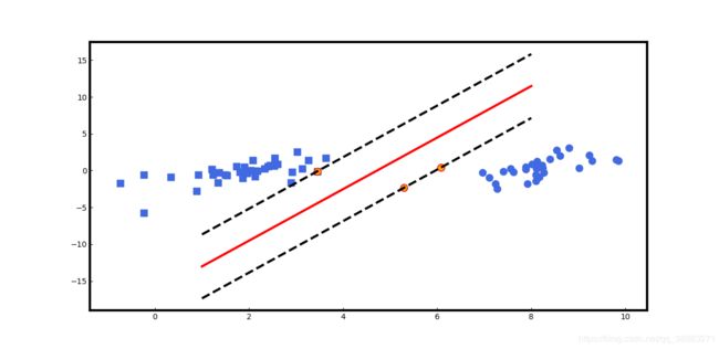
Train Accuracy:1.0000

Test  Accuracy:1.0000
-
数据集非线性可分
此时不能再使用线性核函数,使用线性核函数的错误率会大大增加,应当使用RBF径向基核函数。
from sklearn import svm
from sklearn.model_selection import train_test_split
import numpy as np
from sklearn import metrics
import matplotlib.pyplot as plt

def loadDataSet(filename, delim="\t"):
    f = open(filename)
    stringArr = [line.strip().split(delim) for line in f.readlines()]
    datArr = [list(map(float, line))for line in stringArr]
    return np.mat(datArr)

def svc_classification(dataMat):
    x = dataMat[:, :2]
    y = dataMat[:, 2]

    #划分出训练集和测试集,测试集占总样本30%
    x_train, x_test, y_train, y_test = train_test_split(x, y, test_size=0.3)
    clf = svm.SVC(kernel="rbf")  #选用线性核函数,通过构造函数SVC生成支持向量机对象
    clf.fit(x_train, y_train)     #训练数据集
    pre_train = clf.predict(x_train)    #得到模型关于训练数据集的分类结果
    pre_test = clf.predict(x_test)      #得到模型关于测试数据集的分类结果

    #获取准确度,即正确分类样本占总训练数据集或测试数据集的比例
    print("Train Accuracy:%.4f\n" % metrics.accuracy_score(y_train, pre_train))
    print("Test  Accuracy:%.4f\n" % metrics.accuracy_score(y_test, pre_test))

    #只有线性核函数才能获得coef_,即w^Tx+b=0的w平面系数矩阵
    return x_train, y_train, clf.support_vectors_

if __name__=="__main__":
    dataMat = loadDataSet("testSetRBF2.txt")
    x_train, y_train, support_vectors = svc_classification(dataMat)

    plt.rcParams['xtick.direction'] = 'in'
    plt.rcParams['ytick.direction'] = 'in'

    for i in range(len(x_train)):
        if y_train[i] == 1:
            plt.scatter(x_train[i, 0], x_train[i, 1], marker="^", color="royalblue", s=80)
        else:
            plt.scatter(x_train[i, 0], x_train[i, 1], marker="s", color="royalblue", s=80)

    #标记支持向量机
    for j in range(len(support_vectors)):
        plt.scatter(support_vectors[j, 0], support_vectors[j, 1], marker="o", edgecolors="r", color="orange", s=30)


    ax = plt.gca()
    ax.spines['bottom'].set_linewidth(3)
    ax.spines['left'].set_linewidth(3)
    ax.spines['right'].set_linewidth(3)
    ax.spines['top'].set_linewidth(3)

    plt.show()
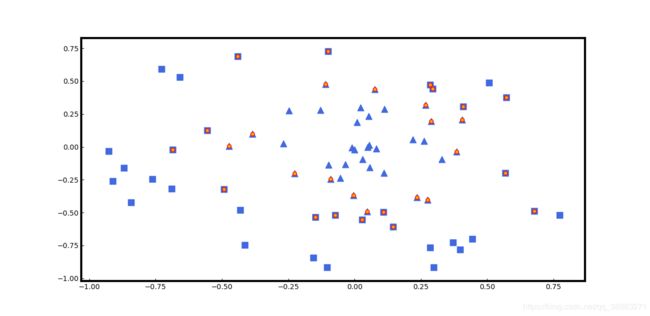
Train Accuracy:0.9857

Test  Accuracy:0.9667
-
利用10折交叉验证进行数据集的训练与测试
from sklearn import svm
from sklearn.model_selection import KFold
import numpy as np
from sklearn import metrics

def loadDataSet(filename, delim="\t"):
    f = open(filename)
    stringArr = [line.strip().split(delim) for line in f.readlines()]
    datArr = [list(map(float, line))for line in stringArr]
    return np.mat(datArr)

def svc_classification(dataMat):
    iter = 1
    x = dataMat[:, :2]
    y = dataMat[:, 2]

    clf = svm.SVC(kernel="rbf")
    kf = KFold(n_splits=10)
    for train, test in kf.split(dataMat):
        clf.fit(x[train, :], y[train, :])     #训练数据集
        pre_train = clf.predict(x[train, :])    #得到模型关于训练数据集的分类结果
        pre_test = clf.predict(x[test, :])      #得到模型关于测试数据集的分类结果

        #获取准确度,即正确分类样本占总训练数据集或测试数据集的比例
        print("The "+str(iter)+"th cross validation:")
        print("Train Accuracy:%.4f" % metrics.accuracy_score(y[train, :], pre_train) + \
              "\tTest  Accuracy:%.4f\n" % metrics.accuracy_score(y[test, :], pre_test))
        iter = iter + 1

if __name__=="__main__":
    dataMat = loadDataSet("testSetRBF2.txt")
    svc_classification(dataMat)
The 1th cross validation:
Train Accuracy:0.9556	Test  Accuracy:1.0000

The 2th cross validation:
Train Accuracy:0.9778	Test  Accuracy:1.0000

The 3th cross validation:
Train Accuracy:0.9778	Test  Accuracy:1.0000

The 4th cross validation:
Train Accuracy:0.9667	Test  Accuracy:0.9000

The 5th cross validation:
Train Accuracy:0.9667	Test  Accuracy:0.9000

The 6th cross validation:
Train Accuracy:0.9667	Test  Accuracy:0.9000

The 7th cross validation:
Train Accuracy:0.9444	Test  Accuracy:1.0000

The 8th cross validation:
Train Accuracy:0.9778	Test  Accuracy:1.0000

The 9th cross validation:
Train Accuracy:0.9778	Test  Accuracy:0.8000

The 10th cross validation:
Train Accuracy:0.9667	Test  Accuracy:0.9000
-
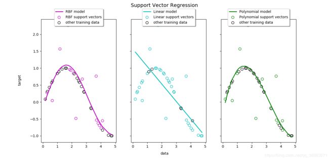
预测模型:
from sklearn import svm
import numpy as np
import matplotlib.pyplot as plt

X = np.sort(5 * np.random.rand(40, 1), axis=0)
y = np.sin(X).ravel()

# 从第一个y开始每5个步长添加噪声数值
y[::5] += 3 * (0.5 - np.random.rand(8))

# epsilon为容忍度,C为正则化惩罚系数,即当预测值与真实值之间的误差大于容忍度时进行L2正则化
# C越大惩罚力度越大,得到的拟合结果越好
# degree为多项式核函数的多项式阶数
svr_rbf = svm.SVR(kernel="rbf", C=100, gamma=0.1, epsilon=.1)
svr_lin = svm.SVR(kernel="linear", C=100, gamma="auto")
svr_poly = svm.SVR(kernel="poly", C=100, gamma="auto", degree=3,\
                   epsilon=.1, coef0=1)

lw = 2   # 线宽
svrs = [svr_rbf, svr_lin, svr_poly]
kernel_label = ['RBF', 'Linear', 'Polynomial']
model_color = ['m', 'c', 'g']

# sharey参数为是否共享纵轴,默认为False
# subplots返回画布(fig)和画布区域(axes)
fig, axes = plt.subplots(nrows=1, ncols=3, figsize=(15, 10), sharey=True)
for ix, svr in enumerate(svrs):
    axes[ix].plot(X, svr.fit(X, y).predict(X), color=model_color[ix], lw=lw,
                  label='{} model'.format(kernel_label[ix]))

    # support_是支持向量机的索引
    axes[ix].scatter(X[svr.support_], y[svr.support_], facecolor="none",
                     edgecolor=model_color[ix], s=50,
                     label='{} support vectors'.format(kernel_label[ix]))

    # 寻找非支持向量机的数据集
    axes[ix].scatter(X[np.setdiff1d(np.arange(len(X)), svr.support_)],
                     y[np.setdiff1d(np.arange(len(X)), svr.support_)],
                     facecolor="none", edgecolor="k", s=50,
                     label='other training data')
    axes[ix].legend(loc='upper center', bbox_to_anchor=(0.5, 1.1),
                    ncol=1, fancybox=True, shadow=True)

fig.text(0.5, 0.04, 'data', ha='center', va='center')
fig.text(0.06, 0.5, 'target', ha='center', va='center', rotation='vertical')
fig.suptitle("Support Vector Regression", fontsize=14)
plt.show()