项目二:Kaggle房价预测(前篇)
概述
Kaggle房价预测比赛(高级技能篇)
notebook的背景是kaggle房价预测比赛高级回归技能篇
背景搬运如下:
这个notebook主要是通过数据探索和数据可视化来实现。
我们把这个过程叫做EDA((Exploratory Data Analysis,探索性数据分析),它往往是比较枯燥乏味的工作。
但是你在理解、清洗和准备数据上花越多的时间,你的预测模型就会越加精准。
- 概述
- 导入库
- 导入数据
- 变量识别
- 统计摘要描述
- 与目标变量的相关性
- 缺失值处理
- 找出含有缺失值的列
- 填充这些缺失值
- 数据可视化
- 单变量分析
- 双变量分析
导入库
import pandas as pd
import numpy as np

import matplotlib.pyplot as plt
% matplotlib inline
import seaborn as sns
sns.set(style="whitegrid", color_codes=True)
sns.set(font_scale=1)
import warnings
warnings.filterwarnings('ignore')
UsageError: Line magic function `%` not found.
导入训练数据集、测试数据
houses=pd.read_csv("./train.csv")
houses.head()
| Id | MSSubClass | MSZoning | LotFrontage | LotArea | Street | Alley | LotShape | LandContour | Utilities | ... | PoolArea | PoolQC | Fence | MiscFeature | MiscVal | MoSold | YrSold | SaleType | SaleCondition | SalePrice | |
|---|---|---|---|---|---|---|---|---|---|---|---|---|---|---|---|---|---|---|---|---|---|
| 0 | 1 | 60 | RL | 65.0 | 8450 | Pave | NaN | Reg | Lvl | AllPub | ... | 0 | NaN | NaN | NaN | 0 | 2 | 2008 | WD | Normal | 208500 |
| 1 | 2 | 20 | RL | 80.0 | 9600 | Pave | NaN | Reg | Lvl | AllPub | ... | 0 | NaN | NaN | NaN | 0 | 5 | 2007 | WD | Normal | 181500 |
| 2 | 3 | 60 | RL | 68.0 | 11250 | Pave | NaN | IR1 | Lvl | AllPub | ... | 0 | NaN | NaN | NaN | 0 | 9 | 2008 | WD | Normal | 223500 |
| 3 | 4 | 70 | RL | 60.0 | 9550 | Pave | NaN | IR1 | Lvl | AllPub | ... | 0 | NaN | NaN | NaN | 0 | 2 | 2006 | WD | Abnorml | 140000 |
| 4 | 5 | 60 | RL | 84.0 | 14260 | Pave | NaN | IR1 | Lvl | AllPub | ... | 0 | NaN | NaN | NaN | 0 | 12 | 2008 | WD | Normal | 250000 |
5 rows × 81 columns
houses_test = pd.read_csv("./test.csv")
houses_test.head()
#注意:这里没有“销售价格”这列,而“销售价格”是我们的目标变量
| Id | MSSubClass | MSZoning | LotFrontage | LotArea | Street | Alley | LotShape | LandContour | Utilities | ... | ScreenPorch | PoolArea | PoolQC | Fence | MiscFeature | MiscVal | MoSold | YrSold | SaleType | SaleCondition | |
|---|---|---|---|---|---|---|---|---|---|---|---|---|---|---|---|---|---|---|---|---|---|
| 0 | 1461 | 20 | RH | 80.0 | 11622 | Pave | NaN | Reg | Lvl | AllPub | ... | 120 | 0 | NaN | MnPrv | NaN | 0 | 6 | 2010 | WD | Normal |
| 1 | 1462 | 20 | RL | 81.0 | 14267 | Pave | NaN | IR1 | Lvl | AllPub | ... | 0 | 0 | NaN | NaN | Gar2 | 12500 | 6 | 2010 | WD | Normal |
| 2 | 1463 | 60 | RL | 74.0 | 13830 | Pave | NaN | IR1 | Lvl | AllPub | ... | 0 | 0 | NaN | MnPrv | NaN | 0 | 3 | 2010 | WD | Normal |
| 3 | 1464 | 60 | RL | 78.0 | 9978 | Pave | NaN | IR1 | Lvl | AllPub | ... | 0 | 0 | NaN | NaN | NaN | 0 | 6 | 2010 | WD | Normal |
| 4 | 1465 | 120 | RL | 43.0 | 5005 | Pave | NaN | IR1 | HLS | AllPub | ... | 144 | 0 | NaN | NaN | NaN | 0 | 1 | 2010 | WD | Normal |
5 rows × 80 columns
#模型命令:展示数据其特征,包括行、样本、例子的数量和列、特征、预测的数量
#(行,列)
houses.shape
(1460, 81)
这里一共有 1460个样本 ,我们可以用这些样本来训练模型,共有 80个特征 和 1个目标变量.
houses_test.shape
#缺少一列,因为目标变量并不在测试区间内
(1459, 80)
识别变量
#info命令,展示数据的相关信息
#包含有每列的总和,空或非空,数据类型,内存占用等
houses.info()
RangeIndex: 1460 entries, 0 to 1459
Data columns (total 81 columns):
Id               1460 non-null int64
MSSubClass       1460 non-null int64
MSZoning         1460 non-null object
LotFrontage      1201 non-null float64
LotArea          1460 non-null int64
Street           1460 non-null object
Alley            91 non-null object
LotShape         1460 non-null object
LandContour      1460 non-null object
Utilities        1460 non-null object
LotConfig        1460 non-null object
LandSlope        1460 non-null object
Neighborhood     1460 non-null object
Condition1       1460 non-null object
Condition2       1460 non-null object
BldgType         1460 non-null object
HouseStyle       1460 non-null object
OverallQual      1460 non-null int64
OverallCond      1460 non-null int64
YearBuilt        1460 non-null int64
YearRemodAdd     1460 non-null int64
RoofStyle        1460 non-null object
RoofMatl         1460 non-null object
Exterior1st      1460 non-null object
Exterior2nd      1460 non-null object
MasVnrType       1452 non-null object
MasVnrArea       1452 non-null float64
ExterQual        1460 non-null object
ExterCond        1460 non-null object
Foundation       1460 non-null object
BsmtQual         1423 non-null object
BsmtCond         1423 non-null object
BsmtExposure     1422 non-null object
BsmtFinType1     1423 non-null object
BsmtFinSF1       1460 non-null int64
BsmtFinType2     1422 non-null object
BsmtFinSF2       1460 non-null int64
BsmtUnfSF        1460 non-null int64
TotalBsmtSF      1460 non-null int64
Heating          1460 non-null object
HeatingQC        1460 non-null object
CentralAir       1460 non-null object
Electrical       1459 non-null object
1stFlrSF         1460 non-null int64
2ndFlrSF         1460 non-null int64
LowQualFinSF     1460 non-null int64
GrLivArea        1460 non-null int64
BsmtFullBath     1460 non-null int64
BsmtHalfBath     1460 non-null int64
FullBath         1460 non-null int64
HalfBath         1460 non-null int64
BedroomAbvGr     1460 non-null int64
KitchenAbvGr     1460 non-null int64
KitchenQual      1460 non-null object
TotRmsAbvGrd     1460 non-null int64
Functional       1460 non-null object
Fireplaces       1460 non-null int64
FireplaceQu      770 non-null object
GarageType       1379 non-null object
GarageYrBlt      1379 non-null float64
GarageFinish     1379 non-null object
GarageCars       1460 non-null int64
GarageArea       1460 non-null int64
GarageQual       1379 non-null object
GarageCond       1379 non-null object
PavedDrive       1460 non-null object
WoodDeckSF       1460 non-null int64
OpenPorchSF      1460 non-null int64
EnclosedPorch    1460 non-null int64
3SsnPorch        1460 non-null int64
ScreenPorch      1460 non-null int64
PoolArea         1460 non-null int64
PoolQC           7 non-null object
Fence            281 non-null object
MiscFeature      54 non-null object
MiscVal          1460 non-null int64
MoSold           1460 non-null int64
YrSold           1460 non-null int64
SaleType         1460 non-null object
SaleCondition    1460 non-null object
SalePrice        1460 non-null int64
dtypes: float64(3), int64(35), object(43)
memory usage: 924.0+ KB
#有多少列具有不同的数据类型?
houses.get_dtype_counts()
float64     3
int64      35
object     43
dtype: int64
##Describe命令,给出数据集中这些数据列的统计信息
houses.describe()
| Id | MSSubClass | LotFrontage | LotArea | OverallQual | OverallCond | YearBuilt | YearRemodAdd | MasVnrArea | BsmtFinSF1 | ... | WoodDeckSF | OpenPorchSF | EnclosedPorch | 3SsnPorch | ScreenPorch | PoolArea | MiscVal | MoSold | YrSold | SalePrice | |
|---|---|---|---|---|---|---|---|---|---|---|---|---|---|---|---|---|---|---|---|---|---|
| count | 1460.000000 | 1460.000000 | 1201.000000 | 1460.000000 | 1460.000000 | 1460.000000 | 1460.000000 | 1460.000000 | 1452.000000 | 1460.000000 | ... | 1460.000000 | 1460.000000 | 1460.000000 | 1460.000000 | 1460.000000 | 1460.000000 | 1460.000000 | 1460.000000 | 1460.000000 | 1460.000000 |
| mean | 730.500000 | 56.897260 | 70.049958 | 10516.828082 | 6.099315 | 5.575342 | 1971.267808 | 1984.865753 | 103.685262 | 443.639726 | ... | 94.244521 | 46.660274 | 21.954110 | 3.409589 | 15.060959 | 2.758904 | 43.489041 | 6.321918 | 2007.815753 | 180921.195890 |
| std | 421.610009 | 42.300571 | 24.284752 | 9981.264932 | 1.382997 | 1.112799 | 30.202904 | 20.645407 | 181.066207 | 456.098091 | ... | 125.338794 | 66.256028 | 61.119149 | 29.317331 | 55.757415 | 40.177307 | 496.123024 | 2.703626 | 1.328095 | 79442.502883 |
| min | 1.000000 | 20.000000 | 21.000000 | 1300.000000 | 1.000000 | 1.000000 | 1872.000000 | 1950.000000 | 0.000000 | 0.000000 | ... | 0.000000 | 0.000000 | 0.000000 | 0.000000 | 0.000000 | 0.000000 | 0.000000 | 1.000000 | 2006.000000 | 34900.000000 |
| 25% | 365.750000 | 20.000000 | 59.000000 | 7553.500000 | 5.000000 | 5.000000 | 1954.000000 | 1967.000000 | 0.000000 | 0.000000 | ... | 0.000000 | 0.000000 | 0.000000 | 0.000000 | 0.000000 | 0.000000 | 0.000000 | 5.000000 | 2007.000000 | 129975.000000 |
| 50% | 730.500000 | 50.000000 | 69.000000 | 9478.500000 | 6.000000 | 5.000000 | 1973.000000 | 1994.000000 | 0.000000 | 383.500000 | ... | 0.000000 | 25.000000 | 0.000000 | 0.000000 | 0.000000 | 0.000000 | 0.000000 | 6.000000 | 2008.000000 | 163000.000000 |
| 75% | 1095.250000 | 70.000000 | 80.000000 | 11601.500000 | 7.000000 | 6.000000 | 2000.000000 | 2004.000000 | 166.000000 | 712.250000 | ... | 168.000000 | 68.000000 | 0.000000 | 0.000000 | 0.000000 | 0.000000 | 0.000000 | 8.000000 | 2009.000000 | 214000.000000 |
| max | 1460.000000 | 190.000000 | 313.000000 | 215245.000000 | 10.000000 | 9.000000 | 2010.000000 | 2010.000000 | 1600.000000 | 5644.000000 | ... | 857.000000 | 547.000000 | 552.000000 | 508.000000 | 480.000000 | 738.000000 | 15500.000000 | 12.000000 | 2010.000000 | 755000.000000 |
8 rows × 38 columns
数据相关性
corr=houses.corr()["SalePrice"]
# print(np.argsort(corr, axis=0))
corr[np.argsort(corr, axis=0)[::-1]]  #np.argsort()表示返回其排序的索引
SalePrice        1.000000
OverallQual      0.790982
GrLivArea        0.708624
GarageCars       0.640409
GarageArea       0.623431
TotalBsmtSF      0.613581
1stFlrSF         0.605852
FullBath         0.560664
TotRmsAbvGrd     0.533723
YearBuilt        0.522897
YearRemodAdd     0.507101
GarageYrBlt      0.486362
MasVnrArea       0.477493
Fireplaces       0.466929
BsmtFinSF1       0.386420
LotFrontage      0.351799
WoodDeckSF       0.324413
2ndFlrSF         0.319334
OpenPorchSF      0.315856
HalfBath         0.284108
LotArea          0.263843
BsmtFullBath     0.227122
BsmtUnfSF        0.214479
BedroomAbvGr     0.168213
ScreenPorch      0.111447
PoolArea         0.092404
MoSold           0.046432
3SsnPorch        0.044584
BsmtFinSF2      -0.011378
BsmtHalfBath    -0.016844
MiscVal         -0.021190
Id              -0.021917
LowQualFinSF    -0.025606
YrSold          -0.028923
OverallCond     -0.077856
MSSubClass      -0.084284
EnclosedPorch   -0.128578
KitchenAbvGr    -0.135907
Name: SalePrice, dtype: float64
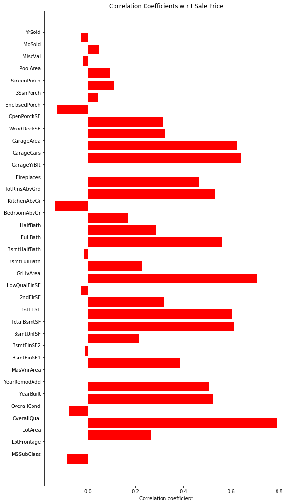
OverallQual ,GrLivArea ,GarageCars,GarageArea ,TotalBsmtSF, 1stFlrSF ,FullBath,TotRmsAbvGrd,YearBuilt, YearRemodAdd 这些变量与SalePrice销售价格的相关性大于0.5
EnclosedPorch and KitchenAbvGr这些变量与SalePrice销售价格的相关性呈现轻度负相关
这些变量是有助于预测房价的重要特征。
#绘制相关性图表
num_feat=houses.columns[houses.dtypes!=object]  #house.dtypes!=object表示输出不是object的类型
num_feat=num_feat[1:-1]  #去掉第0项:ID
labels = []
values = []
for col in num_feat:
    labels.append(col)
    values.append(np.corrcoef(houses[col].values, houses.SalePrice.values)[0,1])
#np.corrcoef()计算皮尔逊相关系数,具体解释可以看https://blog.csdn.net/u012162613/article/details/42213883

ind = np.arange(len(labels))
width = 0.9
fig, ax = plt.subplots(figsize=(9,18))
#fig,ax = plt.subplots()的意思是,同时在subplots里建立一个fig对象,建立一个axis对象
# 这样就不用先plt.figure()
# 再plt.add_subplot()了

rects = ax.barh(ind, np.array(values), color='red')  #ax.barh表示水平条状图
ax.set_yticks(ind+((width)/2.)) #设置y轴刻度宽度
ax.set_yticklabels(labels, rotation='horizontal')  #设置y轴标签
ax.set_xlabel("Correlation coefficient")
ax.set_title("Correlation Coefficients w.r.t Sale Price");
correlations=houses.corr()
# print(correlations)
attrs = correlations.iloc[:-1,:-1] #目标变量除外的所有列

threshold = 0.5

#unstack()表示降维dataframe,转换为行列形式,默认level=-1
important_corrs = (attrs[abs(attrs) > threshold][attrs != 1.0]) \
    .unstack().dropna().to_dict()


#将得到的数据进行重新排序,并生成相关性的dataframe
unique_important_corrs = pd.DataFrame(
    list(set([(tuple(sorted(key)),important_corrs[key]) for key in important_corrs])),
        columns=['Attribute Pair', 'Correlation'])


#以绝对值进行分类排序
unique_important_corrs = unique_important_corrs.iloc[
    abs(unique_important_corrs['Correlation']).argsort()[::-1]]

unique_important_corrs
| Attribute Pair | Correlation | |
|---|---|---|
| 16 | (GarageArea, GarageCars) | 0.882475 |
| 17 | (GarageYrBlt, YearBuilt) | 0.825667 |
| 4 | (GrLivArea, TotRmsAbvGrd) | 0.825489 |
| 1 | (1stFlrSF, TotalBsmtSF) | 0.819530 |
| 26 | (2ndFlrSF, GrLivArea) | 0.687501 |
| 6 | (BedroomAbvGr, TotRmsAbvGrd) | 0.676620 |
| 2 | (BsmtFinSF1, BsmtFullBath) | 0.649212 |
| 25 | (GarageYrBlt, YearRemodAdd) | 0.642277 |
| 15 | (FullBath, GrLivArea) | 0.630012 |
| 14 | (2ndFlrSF, TotRmsAbvGrd) | 0.616423 |
| 20 | (2ndFlrSF, HalfBath) | 0.609707 |
| 23 | (GarageCars, OverallQual) | 0.600671 |
| 9 | (GrLivArea, OverallQual) | 0.593007 |
| 8 | (YearBuilt, YearRemodAdd) | 0.592855 |
| 10 | (GarageCars, GarageYrBlt) | 0.588920 |
| 7 | (OverallQual, YearBuilt) | 0.572323 |
| 12 | (1stFlrSF, GrLivArea) | 0.566024 |
| 5 | (GarageArea, GarageYrBlt) | 0.564567 |
| 21 | (GarageArea, OverallQual) | 0.562022 |
| 24 | (FullBath, TotRmsAbvGrd) | 0.554784 |
| 0 | (OverallQual, YearRemodAdd) | 0.550684 |
| 11 | (FullBath, OverallQual) | 0.550600 |
| 18 | (GarageYrBlt, OverallQual) | 0.547766 |
| 22 | (GarageCars, YearBuilt) | 0.537850 |
| 13 | (OverallQual, TotalBsmtSF) | 0.537808 |
| 27 | (BsmtFinSF1, TotalBsmtSF) | 0.522396 |
| 19 | (BedroomAbvGr, GrLivArea) | 0.521270 |
| 3 | (2ndFlrSF, BedroomAbvGr) | 0.502901 |
这显示了多重共线性。
在线性回归模型中,多重共线性是指特征与其他多个特征相关。当你的模型包含有多个与目标变量相关的因素,而这些因素也相关影响时,即为多重共线性发生。
问题:
多重共线性会增加了这些系数的标准误差。
这意味着,多重共线性会使一些本应该显著的变量,变得没有那么显著。
三种方式可避免这种情况:
- 完全删除这些变量
- 通过添加或一些操作,增加新的特征变量
- 通过PCA(Principal Component Analysis,主成分分析), 来减少特征变量的多重共线性.
参考:http://blog.minitab.com/blog/understanding-statistics/handling-multicollinearity-in-regression-analysis
热力图
import seaborn as sns
corrMatrix=houses[["SalePrice","OverallQual","GrLivArea","GarageCars",
                  "GarageArea","GarageYrBlt","TotalBsmtSF","1stFlrSF","FullBath",
                  "TotRmsAbvGrd","YearBuilt","YearRemodAdd"]].corr()

sns.set(font_scale=1.10)  #font_scale表示图像与字体大小比例
plt.figure(figsize=(10, 10))

sns.heatmap(corrMatrix, vmax=.8, linewidths=0.01,
            square=True,annot=True,cmap='viridis',linecolor="white")
plt.title('Correlation between features');
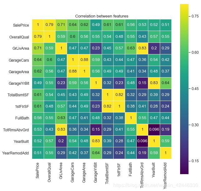
如我们所见,热力图中只有少量特征变量表现出显著的多重共线性。让我们聚焦到对角线的黄色方块和线框出的少量黄色区域。
SalePrice and OverallQual
GarageArea and GarageCars
TotalBsmtSF and 1stFlrSF
GrLiveArea and TotRmsAbvGrd
YearBulit and GarageYrBlt
在我们用这些变量进行预测之前,我们不得不新建一个源于这些变量的单特征变量
关键特征
houses[['OverallQual','SalePrice']].groupby(['OverallQual'],
as_index=False).mean().sort_values(by='OverallQual', ascending=False)
| OverallQual | SalePrice | |
|---|---|---|
| 9 | 10 | 438588.388889 |
| 8 | 9 | 367513.023256 |
| 7 | 8 | 274735.535714 |
| 6 | 7 | 207716.423197 |
| 5 | 6 | 161603.034759 |
| 4 | 5 | 133523.347607 |
| 3 | 4 | 108420.655172 |
| 2 | 3 | 87473.750000 |
| 1 | 2 | 51770.333333 |
| 0 | 1 | 50150.000000 |
houses[['GarageCars','SalePrice']].groupby(['GarageCars'],
as_index=False).mean().sort_values(by='GarageCars', ascending=False)
| GarageCars | SalePrice | |
|---|---|---|
| 4 | 4 | 192655.800000 |
| 3 | 3 | 309636.121547 |
| 2 | 2 | 183851.663835 |
| 1 | 1 | 128116.688347 |
| 0 | 0 | 103317.283951 |
houses[['Fireplaces','SalePrice']].groupby(['Fireplaces'],
as_index=False).mean().sort_values(by='Fireplaces', ascending=False)
| Fireplaces | SalePrice | |
|---|---|---|
| 3 | 3 | 252000.000000 |
| 2 | 2 | 240588.539130 |
| 1 | 1 | 211843.909231 |
| 0 | 0 | 141331.482609 |
目标变量的可视化
单变量分析
1个单变量是如何分布在一个数值区间上。
它的统计特征是什么。
它是正偏分布,还是负偏分布。
sns.distplot(houses['SalePrice'], color="r", kde=False)
plt.title("Distribution of Sale Price")
plt.ylabel("Number of Occurences")
plt.xlabel("Sale Price");
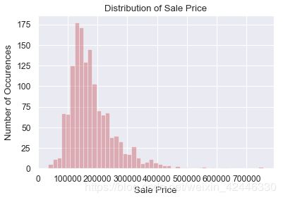
售价为正偏分布,图表显示了一些峰度。
#偏度,表示在请求的轴上返回无偏倾斜
# 具体参考https:https://blog.csdn.net/colorknight/article/details/9531437

houses['SalePrice'].skew()
1.8828757597682129
#峰度,表示使用费雪的峰度定义在请求的轴上返回无偏峰度

houses['SalePrice'].kurt()
6.536281860064529
#删除异常值
#np.percentile()沿着指定的轴计算数据的第q百分位数
upperlimit = np.percentile(houses.SalePrice.values, 99.5)
print(upperlimit)
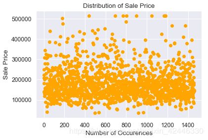
houses['SalePrice'].loc[houses['SalePrice']>upperlimit] = upperlimit
plt.scatter(range(houses.shape[0]), houses["SalePrice"].values,color='orange')
plt.title("Distribution of Sale Price")
plt.xlabel("Number of Occurences")
plt.ylabel("Sale Price");
514508.61012787104
缺失值处理
====================
训练数据集中的缺失值可能会对模型的预测或分类产生负面影响。
有一些机器学习算法对数据缺失敏感,例如支持向量机 SVM(Support Vector Machine)
但是使用平均数/中位数/众数来填充缺失值或使用其他预测模型来预测缺失值也不可能实现100%准确预测,比较可取的方式是你可以使用决策树和随机森林等模型来处理缺失值。
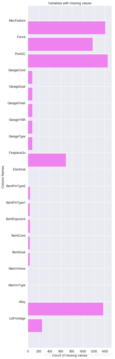
# 查看是否有有缺失值的列
null_columns=houses.columns[houses.isnull().any()]  #.any()表示是否所有元素为真
#得到null_columns为一个含空值的列的list
houses[null_columns].isnull().sum()
LotFrontage      259
Alley           1369
MasVnrType         8
MasVnrArea         8
BsmtQual          37
BsmtCond          37
BsmtExposure      38
BsmtFinType1      37
BsmtFinType2      38
Electrical         1
FireplaceQu      690
GarageType        81
GarageYrBlt       81
GarageFinish      81
GarageQual        81
GarageCond        81
PoolQC          1453
Fence           1179
MiscFeature     1406
dtype: int64
labels = []
values = []
for col in null_columns:
    labels.append(col)
    values.append(houses[col].isnull().sum())
ind = np.arange(len(labels))
width = 0.9
fig, ax = plt.subplots(figsize=(6,25))
rects = ax.barh(ind, np.array(values), color='violet')
ax.set_yticks(ind+((width)/2.))
ax.set_yticklabels(labels, rotation='horizontal')
ax.set_xlabel("Count of missing values")
ax.set_ylabel("Column Names")
ax.set_title("Variables with missing values");
多变量分析
当我们去理解3个及以上变量之间的相互影响。
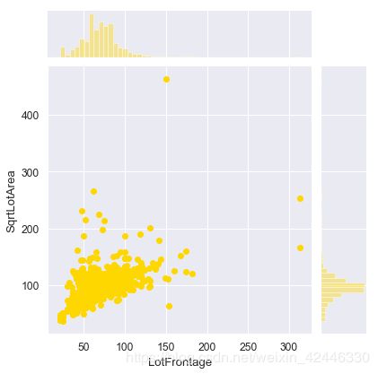
临街距离
我们可以看看占地面积和临街距离之间是否存在某种关联。
houses['LotFrontage'].corr(houses['LotArea'])
0.42609501877180816
这看起来不好,我们可以试试一些多项式表达式,如平方根
houses['SqrtLotArea']=np.sqrt(houses['LotArea'])
houses['LotFrontage'].corr(houses['SqrtLotArea'])
0.6020022167939364
0.60看起来不错
sns.jointplot(houses['LotFrontage'],houses['SqrtLotArea'],color='gold');
filter = houses['LotFrontage'].isnull()
houses.LotFrontage[filter]=houses.SqrtLotArea[filter]
houses.LotFrontage
C:\ProgramData\Anaconda3\lib\site-packages\ipykernel_launcher.py:2: SettingWithCopyWarning:
A value is trying to be set on a copy of a slice from a DataFrame

See the caveats in the documentation: http://pandas.pydata.org/pandas-docs/stable/indexing.html#indexing-view-versus-copy


0        65.000000
1        80.000000
2        68.000000
3        60.000000
4        84.000000
5        85.000000
6        75.000000
7       101.892100
8        51.000000
9        50.000000
10       70.000000
11       85.000000
12      113.877127
13       91.000000
14      104.498804
15       51.000000
16      106.023582
17       72.000000
18       66.000000
19       70.000000
20      101.000000
21       57.000000
22       75.000000
23       44.000000
24       90.807489
25      110.000000
26       60.000000
27       98.000000
28       47.000000
29       60.000000
           ...
1430     60.000000
1431     70.199715
1432     60.000000
1433     93.000000
1434     80.000000
1435     80.000000
1436     60.000000
1437     96.000000
1438     90.000000
1439     80.000000
1440     79.000000
1441     66.528190
1442     85.000000
1443     94.095696
1444     63.000000
1445     70.000000
1446    161.684879
1447     80.000000
1448     70.000000
1449     21.000000
1450     60.000000
1451     78.000000
1452     35.000000
1453     90.000000
1454     62.000000
1455     62.000000
1456     85.000000
1457     66.000000
1458     68.000000
1459     75.000000
Name: LotFrontage, Length: 1460, dtype: float64
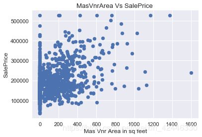
砌体单板类型 and 砌体单板面积
plt.scatter(houses["MasVnrArea"],houses["SalePrice"])
plt.title("MasVnrArea Vs SalePrice ")
plt.ylabel("SalePrice")
plt.xlabel("Mas Vnr Area in sq feet");
sns.boxplot("MasVnrType","SalePrice",data=houses);
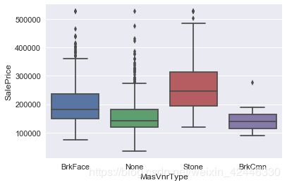
houses["MasVnrType"] = houses["MasVnrType"].fillna('None')
houses["MasVnrArea"] = houses["MasVnrArea"].fillna(0.0)
双变量分析
我们可以尝试去找出数据集中的2个参数是如何相互关联的。 从某种意义上说,当一个参数减少时,另一个参数也减少,或者当一个参数增加时,另一个参数也增加,即为正相关
当一个参数增加,另一个参数减少,或者反之亦然,即为负相关。
电气系统
sns.boxplot("Electrical","SalePrice",data=houses)
plt.title("Electrical Vs SalePrice ")
plt.ylabel("SalePrice")
plt.xlabel("Electrical");
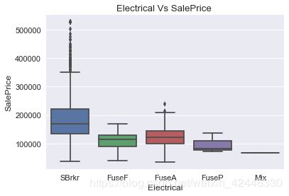
#我们可以用最常见的数值去替代缺失值。
houses["Electrical"] = houses["Electrical"].fillna('SBrkr')
小巷
sns.stripplot(x=houses["Alley"], y=houses["SalePrice"],jitter=True);
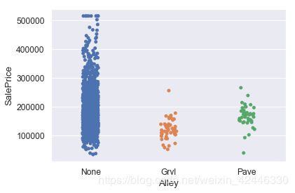
所有缺失值表示特定房屋没有小巷入口。我们可以用’None’来替代。
houses["Alley"] = houses["Alley"].fillna('None')
地下室特征
plt.scatter(houses["TotalBsmtSF"],houses["SalePrice"])
plt.title("Total Basement area in Square Feet Vs SalePrice ")
plt.ylabel("SalePrice")
plt.xlabel("Total Basement area in Square Feet");
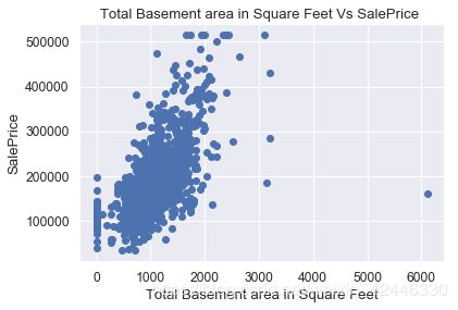
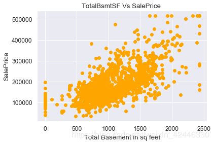
#地下室总面积,有几个的异常值,让我们去除这些值
upperlimit = np.percentile(houses.TotalBsmtSF.values, 99.5)
houses['TotalBsmtSF'].loc[houses['TotalBsmtSF']>upperlimit] = upperlimit

plt.scatter(houses.TotalBsmtSF, houses["SalePrice"].values,color='orange')
plt.title("TotalBsmtSF Vs SalePrice ")
plt.ylabel("SalePrice")
plt.xlabel("Total Basement in sq feet");
basement_cols=['BsmtQual','BsmtCond','BsmtExposure','BsmtFinType1','BsmtFinType2','BsmtFinSF1','BsmtFinSF2']
houses[basement_cols][houses['BsmtQual'].isnull()==True]
| BsmtQual | BsmtCond | BsmtExposure | BsmtFinType1 | BsmtFinType2 | BsmtFinSF1 | BsmtFinSF2 | |
|---|---|---|---|---|---|---|---|
| 17 | NaN | NaN | NaN | NaN | NaN | 0 | 0 |
| 39 | NaN | NaN | NaN | NaN | NaN | 0 | 0 |
| 90 | NaN | NaN | NaN | NaN | NaN | 0 | 0 |
| 102 | NaN | NaN | NaN | NaN | NaN | 0 | 0 |
| 156 | NaN | NaN | NaN | NaN | NaN | 0 | 0 |
| 182 | NaN | NaN | NaN | NaN | NaN | 0 | 0 |
| 259 | NaN | NaN | NaN | NaN | NaN | 0 | 0 |
| 342 | NaN | NaN | NaN | NaN | NaN | 0 | 0 |
| 362 | NaN | NaN | NaN | NaN | NaN | 0 | 0 |
| 371 | NaN | NaN | NaN | NaN | NaN | 0 | 0 |
| 392 | NaN | NaN | NaN | NaN | NaN | 0 | 0 |
| 520 | NaN | NaN | NaN | NaN | NaN | 0 | 0 |
| 532 | NaN | NaN | NaN | NaN | NaN | 0 | 0 |
| 533 | NaN | NaN | NaN | NaN | NaN | 0 | 0 |
| 553 | NaN | NaN | NaN | NaN | NaN | 0 | 0 |
| 646 | NaN | NaN | NaN | NaN | NaN | 0 | 0 |
| 705 | NaN | NaN | NaN | NaN | NaN | 0 | 0 |
| 736 | NaN | NaN | NaN | NaN | NaN | 0 | 0 |
| 749 | NaN | NaN | NaN | NaN | NaN | 0 | 0 |
| 778 | NaN | NaN | NaN | NaN | NaN | 0 | 0 |
| 868 | NaN | NaN | NaN | NaN | NaN | 0 | 0 |
| 894 | NaN | NaN | NaN | NaN | NaN | 0 | 0 |
| 897 | NaN | NaN | NaN | NaN | NaN | 0 | 0 |
| 984 | NaN | NaN | NaN | NaN | NaN | 0 | 0 |
| 1000 | NaN | NaN | NaN | NaN | NaN | 0 | 0 |
| 1011 | NaN | NaN | NaN | NaN | NaN | 0 | 0 |
| 1035 | NaN | NaN | NaN | NaN | NaN | 0 | 0 |
| 1045 | NaN | NaN | NaN | NaN | NaN | 0 | 0 |
| 1048 | NaN | NaN | NaN | NaN | NaN | 0 | 0 |
| 1049 | NaN | NaN | NaN | NaN | NaN | 0 | 0 |
| 1090 | NaN | NaN | NaN | NaN | NaN | 0 | 0 |
| 1179 | NaN | NaN | NaN | NaN | NaN | 0 | 0 |
| 1216 | NaN | NaN | NaN | NaN | NaN | 0 | 0 |
| 1218 | NaN | NaN | NaN | NaN | NaN | 0 | 0 |
| 1232 | NaN | NaN | NaN | NaN | NaN | 0 | 0 |
| 1321 | NaN | NaN | NaN | NaN | NaN | 0 | 0 |
| 1412 | NaN | NaN | NaN | NaN | NaN | 0 | 0 |
所有的包含有NAN的分类变量,含有0值的连续变量。
意味着这些房屋没有地下室。
我们可以用’None’来替代。
for col in basement_cols:
    if 'FinSF'not in col:
        houses[col] = houses[col].fillna('None')
壁炉
#之前的sns.factorplot()不可用了,用catplot()代替,hue表示加入第三个维度的参数
sns.catplot(x="Fireplaces",y="SalePrice",data=houses,hue='FireplaceQu',kind='point');
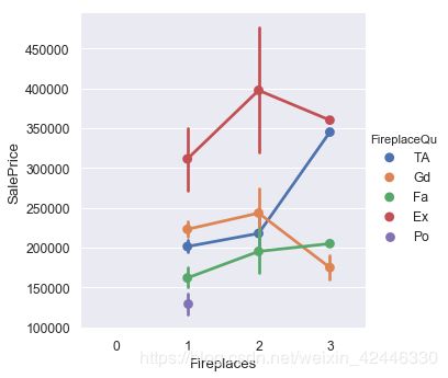
有2个壁炉可以提升房价,优质壁炉也是一大卖点。
#如果壁炉质量存在缺失值,意味着房屋没有壁炉
houses["FireplaceQu"] = houses["FireplaceQu"].fillna('None')
pd.crosstab(houses.Fireplaces, houses.FireplaceQu)
#pd.crosstab()表示计算几个简单因子出现频次的交叉表
| FireplaceQu | Ex | Fa | Gd | None | Po | TA |
|---|---|---|---|---|---|---|
| Fireplaces | ||||||
| 0 | 0 | 0 | 0 | 690 | 0 | 0 |
| 1 | 19 | 28 | 324 | 0 | 20 | 259 |
| 2 | 4 | 4 | 54 | 0 | 0 | 53 |
| 3 | 1 | 1 | 2 | 0 | 0 | 1 |
车库
sns.distplot(houses["GarageArea"],color='r', kde=False);
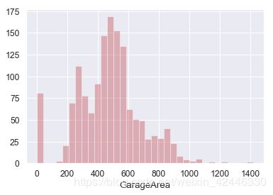
#车库面积存在一些异常值,去除这些异常值(套路代码)
upperlimit = np.percentile(houses.GarageArea.values, 99.5)
houses['GarageArea'].loc[houses['GarageArea']>upperlimit] = upperlimit
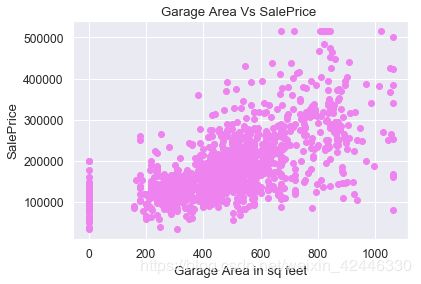
plt.scatter(houses.GarageArea, houses["SalePrice"].values,color='violet')
plt.title("Garage Area Vs SalePrice ")
plt.ylabel("SalePrice")
plt.xlabel("Garage Area in sq feet");
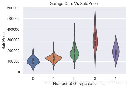
sns.violinplot(houses["GarageCars"],houses["SalePrice"])
plt.title("Garage Cars Vs SalePrice ")
plt.ylabel("SalePrice")
plt.xlabel("Number of Garage cars");
garage_cols=['GarageType','GarageQual','GarageCond','GarageYrBlt','GarageFinish','GarageCars','GarageArea']
houses[garage_cols][houses['GarageType'].isnull()==True]
| GarageType | GarageQual | GarageCond | GarageYrBlt | GarageFinish | GarageCars | GarageArea | |
|---|---|---|---|---|---|---|---|
| 39 | NaN | NaN | NaN | NaN | NaN | 0 | 0.0 |
| 48 | NaN | NaN | NaN | NaN | NaN | 0 | 0.0 |
| 78 | NaN | NaN | NaN | NaN | NaN | 0 | 0.0 |
| 88 | NaN | NaN | NaN | NaN | NaN | 0 | 0.0 |
| 89 | NaN | NaN | NaN | NaN | NaN | 0 | 0.0 |
| 99 | NaN | NaN | NaN | NaN | NaN | 0 | 0.0 |
| 108 | NaN | NaN | NaN | NaN | NaN | 0 | 0.0 |
| 125 | NaN | NaN | NaN | NaN | NaN | 0 | 0.0 |
| 127 | NaN | NaN | NaN | NaN | NaN | 0 | 0.0 |
| 140 | NaN | NaN | NaN | NaN | NaN | 0 | 0.0 |
| 148 | NaN | NaN | NaN | NaN | NaN | 0 | 0.0 |
| 155 | NaN | NaN | NaN | NaN | NaN | 0 | 0.0 |
| 163 | NaN | NaN | NaN | NaN | NaN | 0 | 0.0 |
| 165 | NaN | NaN | NaN | NaN | NaN | 0 | 0.0 |
| 198 | NaN | NaN | NaN | NaN | NaN | 0 | 0.0 |
| 210 | NaN | NaN | NaN | NaN | NaN | 0 | 0.0 |
| 241 | NaN | NaN | NaN | NaN | NaN | 0 | 0.0 |
| 250 | NaN | NaN | NaN | NaN | NaN | 0 | 0.0 |
| 287 | NaN | NaN | NaN | NaN | NaN | 0 | 0.0 |
| 291 | NaN | NaN | NaN | NaN | NaN | 0 | 0.0 |
| 307 | NaN | NaN | NaN | NaN | NaN | 0 | 0.0 |
| 375 | NaN | NaN | NaN | NaN | NaN | 0 | 0.0 |
| 386 | NaN | NaN | NaN | NaN | NaN | 0 | 0.0 |
| 393 | NaN | NaN | NaN | NaN | NaN | 0 | 0.0 |
| 431 | NaN | NaN | NaN | NaN | NaN | 0 | 0.0 |
| 434 | NaN | NaN | NaN | NaN | NaN | 0 | 0.0 |
| 441 | NaN | NaN | NaN | NaN | NaN | 0 | 0.0 |
| 464 | NaN | NaN | NaN | NaN | NaN | 0 | 0.0 |
| 495 | NaN | NaN | NaN | NaN | NaN | 0 | 0.0 |
| 520 | NaN | NaN | NaN | NaN | NaN | 0 | 0.0 |
| ... | ... | ... | ... | ... | ... | ... | ... |
| 954 | NaN | NaN | NaN | NaN | NaN | 0 | 0.0 |
| 960 | NaN | NaN | NaN | NaN | NaN | 0 | 0.0 |
| 968 | NaN | NaN | NaN | NaN | NaN | 0 | 0.0 |
| 970 | NaN | NaN | NaN | NaN | NaN | 0 | 0.0 |
| 976 | NaN | NaN | NaN | NaN | NaN | 0 | 0.0 |
| 1009 | NaN | NaN | NaN | NaN | NaN | 0 | 0.0 |
| 1011 | NaN | NaN | NaN | NaN | NaN | 0 | 0.0 |
| 1030 | NaN | NaN | NaN | NaN | NaN | 0 | 0.0 |
| 1038 | NaN | NaN | NaN | NaN | NaN | 0 | 0.0 |
| 1096 | NaN | NaN | NaN | NaN | NaN | 0 | 0.0 |
| 1123 | NaN | NaN | NaN | NaN | NaN | 0 | 0.0 |
| 1131 | NaN | NaN | NaN | NaN | NaN | 0 | 0.0 |
| 1137 | NaN | NaN | NaN | NaN | NaN | 0 | 0.0 |
| 1143 | NaN | NaN | NaN | NaN | NaN | 0 | 0.0 |
| 1173 | NaN | NaN | NaN | NaN | NaN | 0 | 0.0 |
| 1179 | NaN | NaN | NaN | NaN | NaN | 0 | 0.0 |
| 1218 | NaN | NaN | NaN | NaN | NaN | 0 | 0.0 |
| 1219 | NaN | NaN | NaN | NaN | NaN | 0 | 0.0 |
| 1234 | NaN | NaN | NaN | NaN | NaN | 0 | 0.0 |
| 1257 | NaN | NaN | NaN | NaN | NaN | 0 | 0.0 |
| 1283 | NaN | NaN | NaN | NaN | NaN | 0 | 0.0 |
| 1323 | NaN | NaN | NaN | NaN | NaN | 0 | 0.0 |
| 1325 | NaN | NaN | NaN | NaN | NaN | 0 | 0.0 |
| 1326 | NaN | NaN | NaN | NaN | NaN | 0 | 0.0 |
| 1337 | NaN | NaN | NaN | NaN | NaN | 0 | 0.0 |
| 1349 | NaN | NaN | NaN | NaN | NaN | 0 | 0.0 |
| 1407 | NaN | NaN | NaN | NaN | NaN | 0 | 0.0 |
| 1449 | NaN | NaN | NaN | NaN | NaN | 0 | 0.0 |
| 1450 | NaN | NaN | NaN | NaN | NaN | 0 | 0.0 |
| 1453 | NaN | NaN | NaN | NaN | NaN | 0 | 0.0 |
81 rows × 7 columns
所有与车库相关的变量在同一行存在缺失值。
意味着我们可以用None来替代分类变量,用0来替代这些连续变量。
#套路代码,填充空值
for col in garage_cols:
    if houses[col].dtype==np.object:
        houses[col] = houses[col].fillna('None')
    else:
        houses[col] = houses[col].fillna(0)
泳池
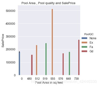
#如果泳池面积为0,则意味这些房屋没有泳池。
#因此,我们可以用None来替代泳池质量。
houses["PoolQC"] = houses["PoolQC"].fillna('None')
sns.catplot("PoolArea","SalePrice",data=houses,hue="PoolQC",kind='bar')
plt.title("Pool Area , Pool quality and SalePrice ")
plt.ylabel("SalePrice")
plt.xlabel("Pool Area in sq feet");
栅栏
sns.violinplot(houses["Fence"],houses["SalePrice"])
plt.title("Fence wrt SalePrice ")
plt.ylabel("SalePrice")
plt.xlabel("Type of Fence");
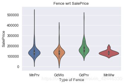
栅栏含有1179个空值。
我们可以确定假设那些房屋没有栅栏,并用None替换这些值。
houses["Fence"] = houses["Fence"].fillna('None')
其他特征
sns.barplot(houses["MiscFeature"],houses["SalePrice"])
plt.title("Miscelleneous Features  Vs SalePrice ")
plt.ylabel("SalePrice")
plt.xlabel("Type of Miscelleneous Features");
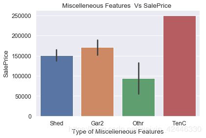
#一些房屋没有其他特征,如棚子、网球场等等
houses["MiscFeature"] = houses["MiscFeature"].fillna('None')
#让我们确认我们已经删除了所有缺失值
houses[null_columns].isnull().sum()
LotFrontage     0
Alley           0
MasVnrType      8
MasVnrArea      8
BsmtQual        0
BsmtCond        0
BsmtExposure    0
BsmtFinType1    0
BsmtFinType2    0
Electrical      0
FireplaceQu     0
GarageType      0
GarageYrBlt     0
GarageFinish    0
GarageQual      0
GarageCond      0
PoolQC          0
Fence           0
MiscFeature     0
dtype: int64
数据可视化
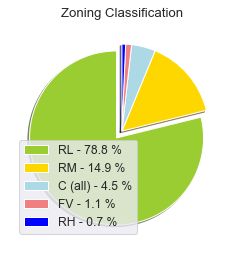
分区划分
美国按照区块划分
labels = houses["MSZoning"].unique()
sizes = houses["MSZoning"].value_counts().values #返回一个统计频次的list
explode=[0.1,0,0,0,0]
parcent = 100.*sizes/sizes.sum()
#zip() 函数用于将可迭代的对象作为参数,将对象中对应的元素打包成一个个元组,然后返回由这些元组组成的列表。
#具体链接:http://www.runoob.com/python/python-func-zip.html
#str.format()具体使用:http://www.runoob.com/python/att-string-format.html
labels = ['{0} - {1:1.1f} %'.format(i,j) for i,j in zip(labels, parcent)]
colors = ['yellowgreen', 'gold', 'lightblue', 'lightcoral','blue']
#explode表示偏移半径
patches, texts= plt.pie(sizes, colors=colors,explode=explode,
shadow=True,startangle=90)
#plt.legend()表示图例,loc表示图例位置
plt.legend(patches, labels, loc="best")
plt.title("Zoning Classification")
plt.show()
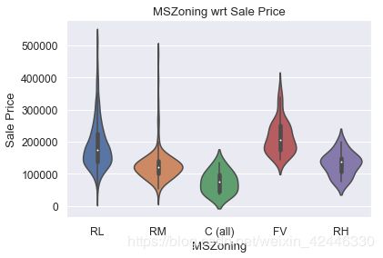
sns.violinplot(houses.MSZoning,houses["SalePrice"])
plt.title("MSZoning wrt Sale Price")
plt.xlabel("MSZoning")
plt.ylabel("Sale Price");
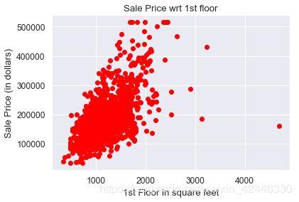
以平方英尺计算的1层面积
plt.scatter(houses["1stFlrSF"],houses.SalePrice, color='red')
plt.title("Sale Price wrt 1st floor")
plt.ylabel('Sale Price (in dollars)')
plt.xlabel("1st Floor in square feet");
houses['1stFlrSF']
0        856
1       1262
2        920
3        961
4       1145
5        796
6       1694
7       1107
8       1022
9       1077
10      1040
11      1182
12       912
13      1494
14      1253
15       854
16      1004
17      1296
18      1114
19      1339
20      1158
21      1108
22      1795
23      1060
24      1060
25      1600
26       900
27      1704
28      1600
29       520
        ...
1430     734
1431     958
1432     968
1433     962
1434    1126
1435    1537
1436     864
1437    1932
1438    1236
1439    1040
1440    1423
1441     848
1442    1026
1443     952
1444    1422
1445     913
1446    1188
1447    1220
1448     796
1449     630
1450     896
1451    1578
1452    1072
1453    1140
1454    1221
1455     953
1456    2073
1457    1188
1458    1078
1459    1256
Name: 1stFlrSF, Length: 1460, dtype: int64
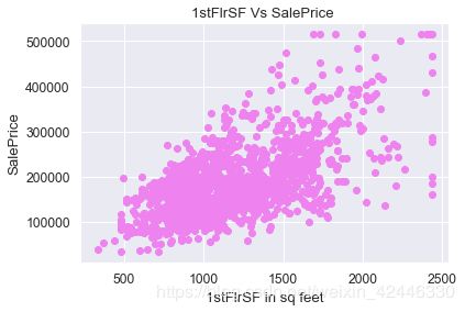
#车库面积存在一些异常值,去除这些异常值(套路代码)
upperlimit = np.percentile(houses['1stFlrSF'].values, 99.5)
houses['1stFlrSF'].loc[houses['1stFlrSF']>upperlimit] = upperlimit

plt.scatter(houses['1stFlrSF'], houses["SalePrice"].values,color='violet')
plt.title("1stFlrSF Vs SalePrice ")
plt.ylabel("SalePrice")
plt.xlabel("1stFlrSF in sq feet");
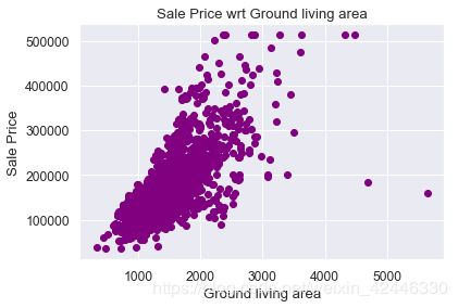
地面生活区的售价
plt.scatter( houses["GrLivArea"],houses["SalePrice"],color='purple')
plt.title("Sale Price wrt Ground living area")
plt.ylabel('Sale Price')
plt.xlabel("Ground living area");
每平方英尺单价
houses['SalePriceSF'] = houses['SalePrice']/houses['GrLivArea']
plt.hist(houses['SalePriceSF'], bins=15,color="gold")  #bin表示柱状图被分割的段数
plt.title("Sale Price per Square Foot")
plt.ylabel('Number of Sales')
plt.xlabel('Price per square feet');
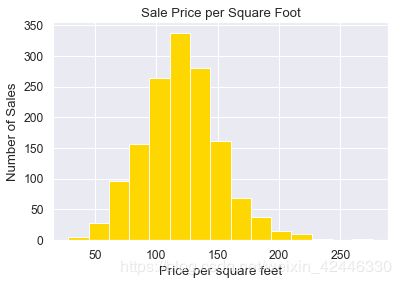
#每平方英尺的平均售价
print("$",houses.SalePriceSF.mean())
$ 120.40732172914129
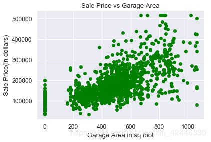
车库面积
plt.scatter(houses["GarageArea"],houses.SalePrice, color='green')
plt.title("Sale Price vs Garage Area")
plt.ylabel('Sale Price(in dollars)')
plt.xlabel("Garage Area in sq foot");
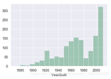
建筑年份,改造年份、房龄
#建筑年份
sns.distplot(houses["YearBuilt"],color='seagreen', kde=False);
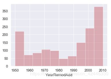
#改造年份
sns.distplot(houses["YearRemodAdd"].astype(int),color='r', kde=False);
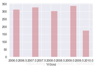
#sold年份
sns.distplot(houses["YrSold"],color='r', kde=False);
#房龄
houses['ConstructionAge'] = houses['YrSold'] - houses['YearBuilt']
plt.scatter(houses['ConstructionAge'], houses['SalePriceSF'])
plt.ylabel('Price per square foot (in dollars)')
plt.xlabel("Construction Age of house");
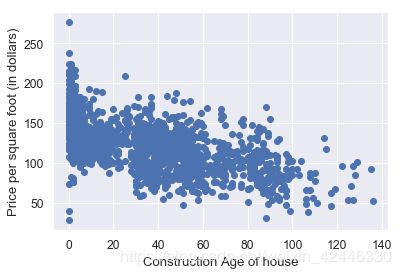
房价与房龄成反比.
暖气和中央空调布置
sns.stripplot(x="HeatingQC", y="SalePrice",data=houses,hue='CentralAir',jitter=True,split=True)
plt.title("Sale Price vs Heating Quality");
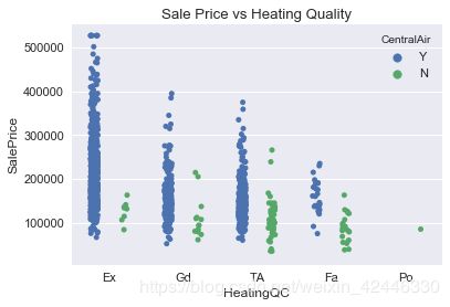
有中央空调布置的房屋,售价更高。
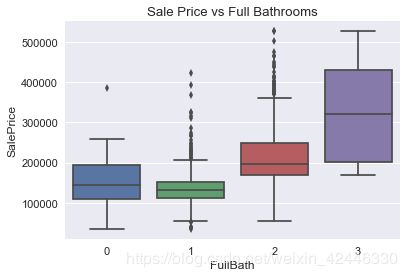
房屋里的浴室
sns.boxplot(houses["FullBath"],houses["SalePrice"])
plt.title("Sale Price vs Full Bathrooms");
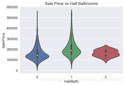
sns.violinplot( houses["HalfBath"],houses["SalePrice"])
plt.title("Sale Price vs Half Bathrooms");
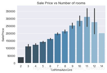
地面以上的总房间数
sns.barplot(houses["TotRmsAbvGrd"],houses["SalePrice"],palette="Blues_d")
plt.title("Sale Price vs Number of rooms");
厨房质量
sns.factorplot("KitchenAbvGr","SalePrice",data=houses,hue="KitchenQual")
plt.title("Sale Price vs Kitchen");
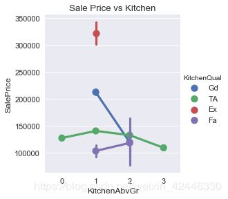
有1个高质量的厨房能够显著的提高房屋售价.
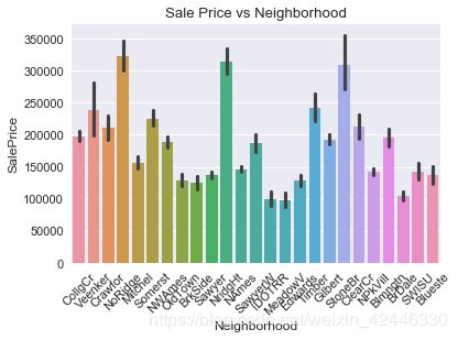
街区
plt.xticks(rotation=45)
sns.barplot(houses["Neighborhood"],houses["SalePrice"])
plt.title("Sale Price vs Neighborhood");
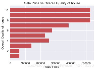
整体质量
plt.barh(houses["OverallQual"],width=houses["SalePrice"],color="r")
plt.title("Sale Price vs Overall Quality of house")
plt.ylabel("Overall Quality of house")
plt.xlabel("Sale Price");
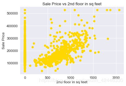
二层售价
plt.scatter(houses["2ndFlrSF"],houses["SalePrice"],color="gold")
plt.title("Sale Price vs 2nd floor in sq feet");
plt.xlabel("2nd floor in sq feet")
plt.ylabel("Sale Price");
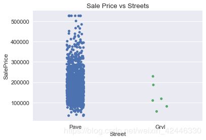
街道
#大多数街道已铺好,让我们可视化它
sns.stripplot(x=houses["Street"], y=houses["SalePrice"],jitter=True)
plt.title("Sale Price vs Streets");
以上只是对数据进行可视化的探索,下次将叙述怎么进行建模和训练,如有错误请大家多多批评。