使用U-Net 进行图像分割
最近做病理AI的细胞计数问题,需要对图像中的各个细胞进行分类,若采用普通的CNN+普通图像分割,估计实现效果不佳。为了解决这个问题,大致有两种方案:目标检测 和 图像分割。目标检测的算法以Faster R-CNN、RetinaNet、YOLO3、SSD等算法为代表;图像分割则以U-Net 等为代表。本文将简述 U-Net。
平时接触较多的是TensorFlow、PyTorch 和 Keras 三大框架,因此本文附上了这三大框架的代码实现。读者可根据自己的习惯选择相应的实现方法。
当然,对于图像分割问题,其实更推荐TensorFlow官方资料:Image Segmentation
注:由于本文大多数内容借鉴自大佬们的博客,而非原创,是故本文为转载类型,参考资料附在了文末。
目录
一、预备知识
1、反卷积操作
2、基于普通CNN实现图像分割
3、FCN(全卷积网络)
二、U-Net介绍
1、基本框架
2、输入输出
3、反向传播
三、U-Net的代码实现
1、PyTorch框架下 U-Net的实现
2、TensorFlow框架下 U-Net的实现
2-1. Layers
2-2. U-Net
3、Keras框架下 U-Net的实现
一、预备知识
1、反卷积操作
本文所介绍的U-Net中关键步骤是上采样,用到了反卷积的知识,具体可参考如下资料。
反卷积(转置卷积)操作(资料1):卷积神经网络CNN(1)——图像卷积与反卷积(后卷积,转置卷积)
反卷积(转置卷积)操作(资料2):Convolution arithmetic tutorial
反卷积本质上可以转化为卷积,下面将卷积操作的概念进行扩展(参考资料:MATLAB二维卷积)。
二维卷积的几种计算形式(shape):1.full 2.same 3. valid
full - 返回完整的二维卷积(如下图)。

same - 返回卷积中大小与 A 相同的中心部分(如下图)。


valid - 仅返回计算的没有补零边缘的卷积部分(如下图)。

2、基于普通CNN实现图像分割
早先,就有人尝试使用传统的CNN框架实现图像分割,2012年NIPS上有一篇论文:Deep Neural Networks Segment Neuronal Membranes in Electron Microscopy Images
思路:对图像的每一个像素点进行分类,在每一个像素点上取一个patch,当做一幅图像,输入神经网络进行训练。
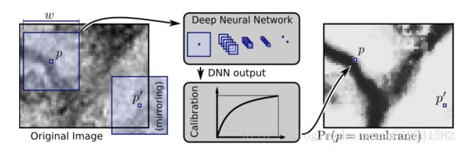
这种网络显然有两个缺点:冗余太大,每个像素点都需取patch,相邻像素点的patch相似度高,网络训练很慢;感受野和定位精度不可兼得。
3、FCN(全卷积网络)
所谓全卷积,就是将原先的全连接层替换成卷积层,使得整个网络的所有层都有卷积操作。
对于图像的语义分割(像素级图像分类),Jonathan Long于2015年发表了《Fully Convolutional Networks for Semantic Segmentation》,使用FCN初步实现了图像分割。这里不详述,请参考相关资料:全卷积网络 FCN 详解
但是到此为止,图像分割并不理想,之后有人在此基础上进行上采样,达到了更精确的分割,这也就是本文所要叙述的U-Net。U-Net是一种特殊的全卷积网络。很多分割网络都是基于FCNs做改进,包括Unet。
二、U-Net介绍
部分内容摘自:Unet 论文解读 代码解读 和 深入理解深度学习分割网络Unet——U-Net: Convolutional Networks for Biomedical Image Segmentation
原论文:http://www.arxiv.org/pdf/1505.04597.pdf
1、基本框架
Unet包括两部分:第一部分,特征提取(convolution layers),与VGG、Inception、ResNet等类似。第二部分上采样部分(upsamping layers)。convolutions layers中每个pooling layer前一刻的activation值会concatenate到对应的upsamping层的activation值中。由于网络结构像U型,所以叫U-Net网络。
- 特征提取部分(convolution layers),每经过一个池化层就一个尺度,包括原图尺度一共有5个尺度。
- 上采样部分(upsamping layers),每上采样一次,就和特征提取部分对应的通道数相同尺度融合,但是融合之前要将其crop。这里的融合也是拼接。
Unet可以采用resnet/vgg/inception+upsampling的形式来实现。

Architecture:
a. U-net建立在FCN的网络架构上,作者修改并扩大了这个网络框架,使其能够使用很少的训练图像就得到很 精确的分割结果。
b.添加上采样阶段,并且添加了很多的特征通道,允许更多的原图像纹理的信息在高分辨率的layers中进行传播。
c. U-net没有FC层,且全程使用valid来进行卷积,这样的话可以保证分割的结果都是基于没有缺失的上下文特征得到的,因此输入输出的图像尺寸不太一样(但是在keras上代码做的都是same convolution),对于图像很大的输入,可以使用overlap-strategy来进行无缝的图像输出。
d.为了预测输入图像的边缘部分,通过镜像输入图像来外推丢失的上下文(不懂),实则输入大图像也是可以的,但是这个策略基于GPU内存不够的情况下所提出的。
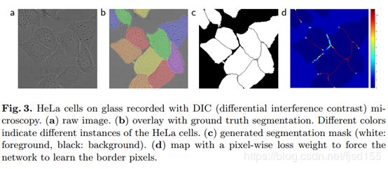
e.细胞分割的另外一个难点在于将相同类别且互相接触的细胞分开,因此作者提出了weighted loss,也就是赋予相互接触的两个细胞之间的background标签更高的权重。

2、输入输出
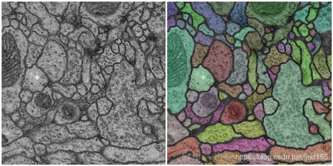
医学图像是一般相当大,但是分割时候不可能将原图太小输入网络,所以必须切成一张一张的小patch,在切成小patch的时候,Unet由于网络结构原因适合有overlap的切图,可以看图,红框是要分割区域,但是在切图时要包含周围区域,overlap另一个重要原因是周围overlap部分可以为分割区域边缘部分提供文理等信息。可以看黄框的边缘,分割结果并没有受到切成小patch而造成分割情况不好。
3、反向传播
Unet反向传播过程,大家都知道卷积层和池化层都能反向传播,Unet上采样部分可以用上采样或反卷积,那反卷积和上采样可以怎么反向传播的呢?由预备知识可知,反卷积(转置卷积)可以转化为卷积操作,因此也是可以反向传播的。
三、U-Net的代码实现
1、PyTorch框架下 U-Net的实现
本部分摘自:用Unet实现图像分割(by pytorch)
采用的是ResNet34+upsampling的架构
class SaveFeatures():
    features=None
    def __init__(self, m): self.hook = m.register_forward_hook(self.hook_fn)
    def hook_fn(self, module, input, output): self.features = output
    def remove(self): self.hook.remove()


class UnetBlock(nn.Module):
  def __init__(self, up_in, down_in, n_out, dp=False, ps=0.25):
    super().__init__()
    up_out = down_out = n_out // 2
    self.tr_conv = nn.ConvTranspose2d(up_in, up_out, 2, 2, bias=False)
    self.conv = nn.Conv2d(down_in, down_out, 1, bias=False)
    self.bn = nn.BatchNorm2d(n_out)
    self.dp = dp
    if dp: self.dropout = nn.Dropout(ps, inplace=True)

  def forward(self, up_x, down_x):
    x1 = self.tr_conv(up_x)
    x2 = self.conv(down_x)
    x = torch.cat([x1, x2], dim=1)
    x = self.bn(F.relu(x))
    return self.dropout(x) if self.dp else x


class Unet34(nn.Module):
  def __init__(self, rn, drop_i=False, ps_i=None, drop_up=False, ps=None):
    super().__init__()
    self.rn = rn
    self.sfs = [SaveFeatures(rn[i]) for i in [2, 4, 5, 6]]
    self.drop_i = drop_i
    if drop_i:
      self.dropout = nn.Dropout(ps_i, inplace=True)
    if ps_i is None: ps_i = 0.1
    if ps is not None: assert len(ps) == 4
    if ps is None: ps = [0.1] * 4
    self.up1 = UnetBlock(512, 256, 256, drop_up, ps[0])
    self.up2 = UnetBlock(256, 128, 256, drop_up, ps[1])
    self.up3 = UnetBlock(256, 64, 256, drop_up, ps[2])
    self.up4 = UnetBlock(256, 64, 256, drop_up, ps[3])
    self.up5 = nn.ConvTranspose2d(256, 1, 2, 2)

  def forward(self, x):
    x = F.relu(self.rn(x))
    x = self.dropout(x) if self.drop_i else x
    x = self.up1(x, self.sfs[3].features)
    x = self.up2(x, self.sfs[2].features)
    x = self.up3(x, self.sfs[1].features)
    x = self.up4(x, self.sfs[0].features)
    x = self.up5(x)
    return x[:, 0]

  def close(self):
    for o in self.sfs: o.remove()
通过注册nn.register_forward_hook() ,将指定resnet34指定层(2, 4, 5, 6)的activation值保存起来,在upsampling的过程中将它们concatnate到相应的upsampling layer中。upsampling layer中使用ConvTranspose2d()来做deconvolution,ConvTranspose2d()的工作机制和conv2d()正好相反,用于增加feature map的grid size
Training
Unet模型训练大致分两步:
- 通过LR Test找出合适的学习率区间。
- Cycle Learning Rate (CLR) 的方法来训练模型,直至过拟合。
wd = 4e-4
arch = resnet34
ps_i = 0.05
ps = np.array([0.1, 0.1, 0.1, 0.1]) * 1
m_base = get_base_model(arch, cut, True)
m = to_gpu(Unet34(m_base, drop_i=True, drop_up=True, ps=ps, ps_i=ps_i))
models = UnetModel(m)
learn = ConvLearner(md, models)
learn.opt_fn = optim.Adam
learn.crit = nn.BCEWithLogitsLoss()
learn.metrics = [accuracy_thresh(0.5), miou]
当模型训练到无法通过变化学习率来减少loss值,val loss收敛且有过拟合的可能时,停止模型的训练。
除了上述代码,网上还有几个不错的实现:
https://github.com/milesial/Pytorch-UNet
http://www.andrewjanowczyk.com/pytorch-unet-for-digital-pathology-segmentation/
https://github.com/ugent-korea/pytorch-unet-segmentation
2、TensorFlow框架下 U-Net的实现
代码来源:https://github.com/jakeret/tf_unet
解读来源:Unet 论文解读 代码解读
2-1. Layers
初始化weights 和 bias
def weight_variable(shape, stddev=0.1, name="weight"):
    initial = tf.truncated_normal(shape, stddev=stddev)
    return tf.Variable(initial, name=name)

def weight_variable_devonc(shape, stddev=0.1, name="weight_devonc"):
    return tf.Variable(tf.truncated_normal(shape, stddev=stddev), name=name)

def bias_variable(shape, name="bias"):
    initial = tf.constant(0.1, shape=shape)
    return tf.Variable(initial, name=name)
创建卷积层和池化层
这里的padding使用的是VALID,和论文里面所指出的是一样的。deconv2d是反卷积,也就是upsampling,以第一个upsample为例,输如的x的shape为[None,28,28,1024],则输出的shape为[None,52,52,512]。反卷积的计算细节参考https://blog.csdn.net/nijiayan123/article/details/79416764。
def conv2d(x, W, b, keep_prob_):
    with tf.name_scope("conv2d"):
        conv_2d = tf.nn.conv2d(x, W, strides=[1, 1, 1, 1], padding='VALID')
        conv_2d_b = tf.nn.bias_add(conv_2d, b)
        return tf.nn.dropout(conv_2d_b, keep_prob_)

def deconv2d(x, W,stride):
    with tf.name_scope("deconv2d"):
        x_shape = tf.shape(x)
        output_shape = tf.stack([x_shape[0], x_shape[1]*2, x_shape[2]*2, x_shape[3]//2])
        return tf.nn.conv2d_transpose(x, W, output_shape, strides=[1, stride, stride, 1], padding='VALID', name="conv2d_transpose")

def max_pool(x,n):
    return tf.nn.max_pool(x, ksize=[1, n, n, 1], strides=[1, n, n, 1], padding='VALID')
连接前面部分的池化层和后面的反卷积层
def crop_and_concat(x1,x2):
    with tf.name_scope("crop_and_concat"):
        x1_shape = tf.shape(x1)
        x2_shape = tf.shape(x2)
        # offsets for the top left corner of the crop
        offsets = [0, (x1_shape[1] - x2_shape[1]) // 2, (x1_shape[2] - x2_shape[2]) // 2, 0]
        size = [-1, x2_shape[1], x2_shape[2], -1]
        x1_crop = tf.slice(x1, offsets, size)
        return tf.concat([x1_crop, x2], 3)
计算pixel-wise softmax和cross entropy
注意到这里一个pixel相当于一个预测目标,在通常的分类任务中,最后输出结果通常都是一个一维向量[1,class_nums],然后取softmax运算后得分最高的class标签。在这里,最后输出结果是一个三维向量[width,height,class_nums],每一个pixel都要单独进行标签的预测,故叫pixel-wise softmax。
def pixel_wise_softmax(output_map):
    with tf.name_scope("pixel_wise_softmax"):
        max_axis = tf.reduce_max(output_map, axis=3, keepdims=True)
        exponential_map = tf.exp(output_map - max_axis)
        normalize = tf.reduce_sum(exponential_map, axis=3, keepdims=True)
        return exponential_map / normalize

def cross_entropy(y_,output_map):
    return -tf.reduce_mean(y_*tf.log(tf.clip_by_value(output_map,1e-10,1.0)), name="cross_entropy")
2-2. U-Net
网络分为四个主要部分:preprocessing、down convolution、up convolution、Output Mappreprocessing
def create_conv_net(x, keep_prob, channels, n_class, layers=3, features_root=16, filter_size=3, pool_size=2,
                    summaries=True):
    """
    Creates a new convolutional unet for the given parametrization.
    :param x: input tensor, shape [?,nx,ny,channels]
    :param keep_prob: dropout probability tensor
    :param channels: number of channels in the input image
    :param n_class: number of output labels
    :param layers: number of layers in the net
    :param features_root: number of features in the first layer
    :param filter_size: size of the convolution filter
    :param pool_size: size of the max pooling operation
    :param summaries: Flag if summaries should be created
    """

    logging.info(
        "Layers {layers}, features {features}, filter size {filter_size}x{filter_size}, pool size: {pool_size}x{pool_size}".format(
            layers=layers,
            features=features_root,
            filter_size=filter_size,
            pool_size=pool_size))

    # Placeholder for the input image
    with tf.name_scope("preprocessing"):
        nx = tf.shape(x)[1]
        ny = tf.shape(x)[2]
        x_image = tf.reshape(x, tf.stack([-1, nx, ny, channels]))
        in_node = x_image
        batch_size = tf.shape(x_image)[0]

    weights = []
    biases = []
    convs = []
    pools = OrderedDict()
    deconv = OrderedDict()
    dw_h_convs = OrderedDict()
    up_h_convs = OrderedDict()

    in_size = 1000
    size = in_size
down convolution
layers=3,有三次下卷积层,一个下卷积层实际包括两次下卷积和一次pooling。
    # down layers
    for layer in range(0, layers):
        with tf.name_scope("down_conv_{}".format(str(layer))):
            features = 2 ** layer * features_root
            stddev = np.sqrt(2 / (filter_size ** 2 * features))
            if layer == 0:
                w1 = weight_variable([filter_size, filter_size, channels, features], stddev, name="w1")
            else:
                w1 = weight_variable([filter_size, filter_size, features // 2, features], stddev, name="w1")

            w2 = weight_variable([filter_size, filter_size, features, features], stddev, name="w2")
            b1 = bias_variable([features], name="b1")
            b2 = bias_variable([features], name="b2")

            conv1 = conv2d(in_node, w1, b1, keep_prob)
            tmp_h_conv = tf.nn.relu(conv1)
            conv2 = conv2d(tmp_h_conv, w2, b2, keep_prob)
            dw_h_convs[layer] = tf.nn.relu(conv2)

            weights.append((w1, w2))
            biases.append((b1, b2))
            convs.append((conv1, conv2))

            size -= 4
            if layer < layers - 1:
                pools[layer] = max_pool(dw_h_convs[layer], pool_size)
                in_node = pools[layer]
                size /= 2

    in_node = dw_h_convs[layers - 1]
up convolution
layers=3,有三次反卷积层,一个反卷积层实际包括一个反卷积,一个连接操作和两次下卷积。
    # up layers
    for layer in range(layers - 2, -1, -1):
        with tf.name_scope("up_conv_{}".format(str(layer))):
            features = 2 ** (layer + 1) * features_root
            stddev = np.sqrt(2 / (filter_size ** 2 * features))

            wd = weight_variable_devonc([pool_size, pool_size, features // 2, features], stddev, name="wd")
            bd = bias_variable([features // 2], name="bd")
            h_deconv = tf.nn.relu(deconv2d(in_node, wd, pool_size) + bd)
            h_deconv_concat = crop_and_concat(dw_h_convs[layer], h_deconv)
            deconv[layer] = h_deconv_concat

            w1 = weight_variable([filter_size, filter_size, features, features // 2], stddev, name="w1")
            w2 = weight_variable([filter_size, filter_size, features // 2, features // 2], stddev, name="w2")
            b1 = bias_variable([features // 2], name="b1")
            b2 = bias_variable([features // 2], name="b2")

            conv1 = conv2d(h_deconv_concat, w1, b1, keep_prob)
            h_conv = tf.nn.relu(conv1)
            conv2 = conv2d(h_conv, w2, b2, keep_prob)
            in_node = tf.nn.relu(conv2)
            up_h_convs[layer] = in_node

            weights.append((w1, w2))
            biases.append((b1, b2))
            convs.append((conv1, conv2))

            size *= 2
            size -= 4
Output Map
    # Output Map
    with tf.name_scope("output_map"):
        weight = weight_variable([1, 1, features_root, n_class], stddev)
        bias = bias_variable([n_class], name="bias")
        conv = conv2d(in_node, weight, bias, tf.constant(1.0))
        output_map = tf.nn.relu(conv)
        up_h_convs["out"] = output_map

    if summaries:
        with tf.name_scope("summaries"):
            for i, (c1, c2) in enumerate(convs):
                tf.summary.image('summary_conv_%02d_01' % i, get_image_summary(c1))
                tf.summary.image('summary_conv_%02d_02' % i, get_image_summary(c2))

            for k in pools.keys():
                tf.summary.image('summary_pool_%02d' % k, get_image_summary(pools[k]))

            for k in deconv.keys():
                tf.summary.image('summary_deconv_concat_%02d' % k, get_image_summary(deconv[k]))

            for k in dw_h_convs.keys():
                tf.summary.histogram("dw_convolution_%02d" % k + '/activations', dw_h_convs[k])

            for k in up_h_convs.keys():
                tf.summary.histogram("up_convolution_%s" % k + '/activations', up_h_convs[k])

    variables = []
    for w1, w2 in weights:
        variables.append(w1)
        variables.append(w2)

    for b1, b2 in biases:
        variables.append(b1)
        variables.append(b2)

    return output_map, variables, int(in_size - size)
3、Keras框架下 U-Net的实现
本部分摘自:全卷积神经网络图像分割(U-net)-keras实现
采用的数据集是一个isbi挑战的数据集,网址为: http://brainiac2.mit.edu/isbi_challenge/
数据集需要注册下载,GitHub上也有下载好的数据集。
这个挑战就是提取出细胞边缘,属于一个二分类问题,问题不算难,可以当做一个练手。
这里最大的挑战就是数据集很小,只有30张512*512的训练图像,所以进行图像增强是非常有必要的。
这里参考了一篇做图像扭曲的论文,http://faculty.cs.tamu.edu/schaefer/research/mls.pdf
进行图像增强的代码: http://download.csdn.net/detail/u012931582/9817058
keras实现: https://github.com/zhixuhao/unet
其它
U-net:运行你的第一个U-net进行图像分割
参考资料
Image Segmentation
Unet 论文解读 代码解读
深入理解深度学习分割网络Unet——U-Net: Convolutional Networks for Biomedical Image Segmentation
全卷积神经网络图像分割(U-net)-keras实现
用Unet实现图像分割(by pytorch)
全卷积网络 FCN 详解
卷积神经网络CNN(1)——图像卷积与反卷积(后卷积,转置卷积)