直方图
直方图简单来说就是图像中每个像素值的个数统计,比如说一副灰度图中像素值为 0 的有多少个,1 的多少个……。直方图是一种分析图片的手段。
Numpy 中直方图计算
其中 ravel() 函数将二维矩阵展平变成一维数组:
from matplotlib import pyplot as plt
import cv2
import numpy as np


def getI(fname, show=False):
    img = plt.imread(fname)
    if show:
        plt.imshow(img)
        plt.show()
    return img


fname = r'E:\Data\URLimg\猫\波斯猫\16.jpg'

img = getI(fname, show=True)
%%time
hist, bins = np.histogram(img[:,:,0].ravel(), 256, [0, 256])  # 性能:26.5 ms
Wall time: 28.5 ms
%%time
hist = np.bincount(img[:,:,0].ravel(), minlength=256)  # 性能:13 ms
Wall time: 10 ms
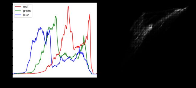
画出直方图
fig, ax = plt.subplots(1, 2, figsize=(12, 5))
colors = ['red', 'green', 'blue']


for i in range(3):
    hist, x = np.histogram(img[:, :, i].ravel(), bins=256, range=(0, 256)) # bins 指定统计区间被等分的个数
    ax[0].plot(.5 * (x[:-1] + x[1:]), hist, label=colors[i], color=colors[i])

ax[0].legend(loc='upper left')
ax[0].set_xlim(0, 256)
hist2, x2, y2 = np.histogram2d(img[:,:,0].ravel(), img[:,:,2].ravel(), bins=(100, 100), range=[(0,256), (0,256)])
ax[1].imshow(hist2, extent=(0, 256, 0, 256), origin='lower', cmap='gray')
ax[1].set_ylabel('red')
ax[1].set_xlabel('blue')
plt.show()
output_5_0.png
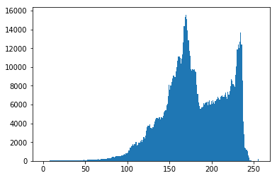
其实 Matplotlib 自带了一个计算并绘制直方图的功能,不需要用到上面的函数:
plt.hist(img[:,:,0].ravel(), 256, [0, 256])
plt.show()
output_7_0.png
OpenCV 中直方图计算
cv2.calcHist(images, channels, mask, histSize, ranges)
-
images:要计算的原图,以方括号的传入,如:[img] -
channels:度图写[0]就行,彩色图B/G/R分别传入[0]/[1]/[2] -
mask:要计算的区域,计算整幅图的话,写None -
histSize:前面提到的bins -
ranges:前面提到的range
%%time
hist = cv2.calcHist([img], [2, 1, 0], None, [30, 20, 10], [0, 256]*3)  # 性能:2.5 ms
Wall time: 3.52 ms
hist.shape
(30, 20, 10)
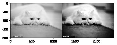
直方图均衡化
一副效果好的图像通常在直方图上的分布比较均匀,直方图均衡化就是用来改善图像的全局亮度和对比度。其实从观感上就可以发现,前面那幅图对比度不高,偏灰白。
OpenCV 中用 cv2.equalizeHist() 实现均衡化。我们把两张图片并排显示,对比一下:
equ = cv2.equalizeHist(img[:,:,0])

plt.imshow(np.hstack((img[:,:,0], equ)), cmap = 'gray')  # 并排显示
plt.show()
output_12_0.png
fig, ax = plt.subplots(1, 2, figsize=(10, 5))

ax[0].hist(img[:,:,0].ravel(), 256, [0, 256])
ax[0].set_title('Hist')
ax[1].hist(equ.ravel(), 256, [0, 256])
ax[1].set_title('equalizeHist')
plt.show()

output_13_0.png
可以看到均衡化后图片的亮度和对比度效果明显好于原图。不难看出来,直方图均衡化是应用于整幅图片的,这样会模糊掉一部分细节信息。自适应均衡化就是用来解决这一问题的:它在每一个小区域内(默认 )进行直方图均衡化。当然,如果有噪点的话,噪点会被放大,需要对小区域内的对比度进行了限制,所以这个算法全称叫:对比度受限的自适应直方图均衡化CLAHE(Contrast Limited Adaptive Histogram Equalization)
自适应均衡化
# 自适应均衡化,参数可选
clahe = cv2.createCLAHE(clipLimit=2.0, tileGridSize=(8, 8))
cl1 = clahe.apply(img[:,:,0])

plt.imshow(np.hstack((img[:,:,0], equ, cl1)), cmap = 'gray')  # 并排显示
plt.show()

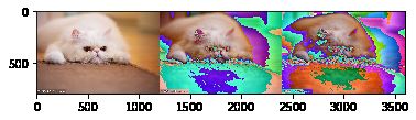
点运算
即对应元素的四则运算:
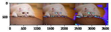
# 乘法
plt.imshow(np.hstack([img*i for i in range(1,4)]))
plt.show()
output_17_0.png
# 除法
plt.imshow(np.hstack([img/i for i in [2, 5, 7]]).astype('B'))
plt.show()

output_18_0.png
# 加法
plt.imshow(np.hstack([img+i for i in [2, 30, 70]]))
plt.show()

output_19_0.png
# 减法
plt.imshow(np.hstack([img-i for i in [2, 50, 70]]).astype('B'))
plt.show()
output_20_0.png
# 组合运算
plt.imshow(np.hstack([img*i-i for i in [2, 50, 70]]).astype('B'))
plt.show()

output_21_0.png
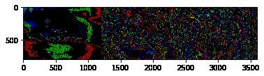
#  指数运算
plt.imshow(np.hstack([np.exp(img*i + 1e-9) for i in [2, 50, 70]]).astype('B'))
plt.show()
output_22_0.png
# 对数运算
plt.imshow(np.hstack([np.log(img*i + 1e-9) for i in [2, 50, 70]]).astype('B'))
plt.show()

output_23_0.png
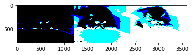
# 阈值处理
plt.imshow(np.hstack([255*(img < i).astype('B') for i in [50, 150, 200]]))
plt.show()
output_24_0.png