Digital Image Processing
- Digital Image Processing---Wavelets
- 1. Introduction
- 2. Related Work
- 2.1 Preliminary knowledge
- 2.2 Background
- 3. Approach
- 3.1 The Fast Wavelet Transform
- 3.1.1 FWTs Using the Wavelet Toolbox
- 3.1.2 FWTs without the Wavelet Toolbox
- 3.2 Working with Wavelet Decomposition Structures
- 3.2.1 Editing Wavelet Decomposition Coefficients without the Wavelet Toolbox
- 3.2.2 Displaying Wavelet Decomposition Coefficients
- 3.3 The Inverse Fast Wavelet Transform
- 3.4 Wavelets in Image Processing
- 4. Experimental Setup
- 4.1 Haar filters, scaling, and wavelet functions.
- 4.2 A simple FWT using Haar filters.
- 4.3 Comparing the execution times ofwavefast and wavedec2.
- 4.4 Wavelet Toolbox functions for manipulating transform decomposition vector c.
- 4.5 Manipulating c with wavecut and wavecopy.
- 4.6 Transform coefficient display using wavedisplay.
- 4.7 Comparing the execution times of waveback and waverec2.
- 4.8 Wavelet directionality and edge detection.
- 4.9 Wavelet-based image smoothing or blurring.
- 4.10 Progressive reconstruction.
- 5. Conclusion
- 6. Appendix
Digital Image Processing—Wavelets
Abstract
The Fourier transform is a beautiful mathematical description, but the computer implementation is discrete step by step from the time domain and the frequency domain.The Fourier transform only shows the frequency properties of the signal or image, and does not provide any time domain information.Wavelet analysis is the latest time - frequency analysis tool.Compared with Fourier transform, discrete wavelet transform inherits and develops the idea of short-time Fourier transform localization and overcomes the disadvantage that the window size does not change with frequency. In addition to being effective and highly intuitive in describing frames and multi-resolution storage, DWT also helps in gaining insight into the spatial and frequency characteristics of images.This paper discusses the calculation and application of discrete wavelet transform.The wavelet toolbox is first introduced.Secondly, the wavelet decomposition structure and fast inverse wavelet transform are studied.Finally, wavelet transform is applied to edge detection, image smoothing and progressive reconstruction.Experimental results show that wavelet transform is widely used in image processing.
1. Introduction
When digital images are to be viewed or processed at multiple resolutions, the discrete wavelet transform (DWT) is the mathematical tool of choice. In addition to being an efficient, highly intuitive framework for the representation and storage of multiresolution images, the DWT provides powerful insight into an image's spatial and frequency characteristics. The Fourier transform, on the other hand, reveals only an image's frequency attributes.
In simple terms, in the traditional Fourier analysis, the signal is completely spread out in the frequency domain, without any time domain information.And has the characteristics of multi-resolution wavelet transform, both in time domain and frequency domain has the ability to characterize local information, time and frequency window can be adjusted according to the concrete forms of signal dynamic, in the low frequency part adopts lower temporal resolution, which improve the resolution of frequency, under the condition of high frequency and low frequency resolution is used to obtain accurate positioning.
In this paper, we explore both the computation and use of the discrete wavelet transform. We introduce the Wavelet Toolbox, a collection of MathWorks' functions designed for wavelet analysis but not included in MATLAB's Image Processing Toolbox, and develop a compatible set of routines that allow wavelet-based processing using the Image Processing Toolbox alone; that is, without the Wavelet Toolbox. These custom functions, in combination with Image Processing Toolbox functions, provide the necessary tools .They are applied in much the same way-and provide a similar range of capabilities-as toolbox functions fft2 and i fft2.Then we study the structure of wavelet decomposition and fast inverse wavelet transform.Finally, we apply wavelet transform to edge detection, image smoothing and progressive reconstruction.
2. Related Work
2.1 Preliminary knowledge
First let us review what a wavelet is ,real word data or signals frequqently exhibit slowly changing trends or oscillations punctuated with transients, on the other hand ,images have smooth regions interrupted by edges or abrupt changes in contrast.These abrupt changes are often the most interesting parts of the data both perceptually and in terms of the information they provide.The Fourier transform is a powerful tool for data analysis ,however it does not represent abrupt changes efficiently .The reason for that is that the Fourier transform represents data as a sum of sine waves which are not localized in time or space,these sine waves oscillate forever.Therefore to accurately analyze signals and images that have abrupt changes ,we need to use a new class of functions that are well localized in time and frequency,this brings us to the topic of wavelets,a wavelet is a rapidly decaying wave like oscillation that has zero mean,unlike sinusoids which extend to infinity ,a wavelet exists for a finite duration,wavelets come in different sizes and shapes.The availability of a wide range of wavelets is a key strength of wavelet analysis ,to choose the right wavelet,you will need to consider the application you will use it for.For now ,let us focus on two important wavelet transform concepts , scaling and shifting ,let us start with scaling ,say you have a signal Sai of T,scaling refers to the process of stretching or shrinking the signal in time which can be expressed using this equation :

s is a scaling factor which is a positive value and corresponds to how much a signal is scaled in time .The scale factor is inversely proportional to frequency.For example,scaling the sine wave by two results in reducing original frequency by half or by octave .For a wavelet,there is a reciprocal relationship between the scale and the frequency with a constant of proportionality.This constant of proportionality is called the center frequency of wavelet.This is because unlike the sine wave,the wavelet has a band pass characteristic ,in the frequency domain ,mathematically ,the equivalent frequency is defined using this equation :

Where CF is the center frequency of the wavelet ,s is the wavelet scale and dalta T is the sampling interval.

Therefore when you scale a wavelet by a factor of 2 ,it results in reducing the equivalent frequency by an octave .A larger scale factor (s>1) results in a stretched wavelet which corresponds to a lower frequency,a smaller scale factor results in a shrunken wavelet which corresponds to a high frequency.A stretched wavelet helps in capturing the slowly varying changes in the signal while a compressed wavelet helps in capturing the abrupt changes.You can construct different scales that inversely correspond to the equivalent frequencies as mentioned earlier.Next we will discuss shifting ,shifting a wavelet simply means delaying or advancing the onset of the wavelet along the length of the signal.

A shifted wavelet represented using this notation means that the wavelet is shifted and centered at K ,we need to shift the wavelet to align with the feature we are looking for in the signal ,the two major transforms in wavelet analysis are continuous and discrete wavelet transforms ,these transforms differ bases on how the wavelets are scaled and shifted,now we have got the basic concepts behind wavelets.
we will now look at two types of wavelet transforms ,the continuous wavelet transform and the discrete wavelet transform.Key applications of continuous wavelet analysis are time frequency analysis and filtering of time localized frequency components.The key applications for discrete wavelet analysis are dennoising and compression of signals and images as mentioned in the previous.This two transforms differ based on how they discretize the scale and the translation parameters .We will discuss these techniques as they apply in the 1d scenario.Let us take a closer look at the continuous wavelet transform or CWT,you can use this transform to obtain a simultaneous time frequency analysis of a signal.Analytic wavelets are best suited for time frequency analysis as these wavelets do not have negative frequency component.
1. Morse Wavelets
2. Bump Wavelet
3. Analytic Morlet Wavelet
This list includes some of the analytic waveletes that are suitable for continous wavelet analysis ,the output of CWT are coefficients which are function of scale or frequency and time.Let us now discuss the process of constructing different wavelet scales,when you scale a wavelet by a factor of 2,it results in reducing the equivalent frequency by an octave .With th e CWT, you have the added flexibility to analyze the signal at intermediary scales within each octave,this allows for fine scale analysis .

This parameter is referred as the number of scales per octave.The higher the number of scales per octave,the finer the scale discretization.Typical values for this parameter are 10,12,16and 32 .The scales are multiplied with the sampling interval of the signal to obtain a physical significance .Here is an example of scales for a bump wavelet with 32 scales per octave .The signal is sampled every 7 microseconds,this is the corresponding plot with the euivalent frequency for the scales,notice that the actual scale values are exponential.Now each scale wavelet is shifted in time along the entire length of the signal and compared with the original signal.You can repeat this process for all the scales resulting in coefficients that are a function of wavelet scale and shift parameter.To put it in perspective,a signal with 1000 samples analyzed with 20 scales results in 20000 coeddicients ,in this way you can better characterize oscillatory behavior in signals with the continuous wavelet transform,the discrete wavalet ransform or DWT is ideal for denoising and compressing signals and images as it help represent many naturally occurring signals and images with fewer coefficients ,this enables a sparser representation.The base scale in dwt is set to 2,you can obtain different scales by raising this base scale to integers values represented in this way .The translation occurs at integer multiples represented in this equation.This process is often referred to as dyadic scaling and shifting ,this kind of sampling eliminates redundacy in coefficients.The output of the transform yields the same number of coefficients as the length of the input signal.Therefore it requires less memory .The discrete wavelet transfrom process is equivalent to comparing a signal with discrete nulti rate filter banks .
Conceptually here is how it works,given a signal s ,the signal is first filtered with special low-pass and high-pass filters to yield low-pass and high-pass sun bands.
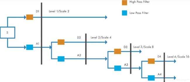
FIGURE 7.1
We can refer to this as a1 and d1 ,half of the samples are discarded after filtering as per the Nyquist criterion .The filters typically have a small number of coefficients and result in good computational performance.These filters also have the led to reconstruct the sub bands while camnceling any aliasing that occurs due to down sampling .For the next level of decomposition,the low-pass sub band a1 is iteratively filtered by the same technique to yield narrower sub bands a2 and d2 and so on,the length of the coefficients in each sub band is half of the number of coefficients in the preceding stage ,the dis technique you can capture the signal of interest with a few large magnitude DWD coefficients while the noise in the signal results in smaller dwt coefficients.This way DWT helps analyze signals at progressively narrower sub bands at different resolution ,it also helps D noise and compress signals .
2.2 Background
Consider an image f(x, y) of size M X N whose forward, discrete transform,T(u,v,...) can be expressed in terms of the general relation:

where x and y are spatial variables and u, v, ... are transform domain variables. Given T(u, v, ... ), f(x, y) can be obtained using the generalized inverse discrete transform :

The g uv.. and h u,v.... in these equations are called forward and inverse tranformation kernels,respectively. They determine the nature, computational complexity, and ultimate usefulness of the transform pair. Transform coefficients T(u, v, ... ) can be viewed as the expansion coefficients of a series expansion of with respect to {h u,v,..} That is, the inverse transformation kernel defines a set of expansion functions for the series expansion of f.
The discrete Fourier transform (DFT) fits this series expansion formulation well. In this case :

where j =√(-1), * is the complex conjugate operator, u = 0, 1, ... , M -1 and v = 0, 1, ... , N -1. Transform domain variables u and v represent horizontal and vertical frequency, respectively. The kernels are separable since:

for


and orthonormal because

where <> is the inner product operator. The separability of the kernels simplifies the computation of the 2-D transform by allowing row-column or columnrow passes of a 1-D transform to be used; orthonormality causes the forward and inverse kernels to be the complex conjugates of one another (they would be identical if the functions were real).
Unlike the discrete Fourier transform, which can be completely defined by two straightforward equations that revolve around a single pair of transformation kernels (given previously), the term discrete wavelet transform refers to a class of transformations that differ not only in the transformation kernels employed (and thus the expansion functions used), but also in the fundamental nature of those functions (e.g., whether they constitute an orthonormal or biorthogonal basis) and in the way in which they are applied (e.g., how many different resolutions are computed). Since the DWT encompasses a variety of unique but related transformations, we cannot write a single equation that completely describes them all. Instead, we characterize each DWT by a transform kernel pair or set of parameters that defines the pair. The various transforms are related by the fact that their expansion functions are "small waves" (hence the name wavelets) of varying frequency and limited duration . In the remainder of the chapter, we introduce a number of these "small wave" kernels. Each possesses the following general properties:
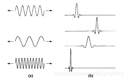
FIGURE 7.2
(a) The familiar Fourier expansion functions are sinusoids of varying frequency and infinite duration. (b) DWT expansion functions are sinusoids of varying frequency and infinite duration.
Property 1: Separability, Scalability, and Translatability. The kernels can be represented as three separable 2-D wavelets :


They are called horizantal, vertical, and diagonal wavelets , respectively, and one separable 2-D scaling function :

Each of these 2-D functions is the product of two 1-D real, square-integrable scaling and wavelet functions :


Translation k determines the position of these 1-D functions along the x-axis, scale j determines their width — how broad or narrow they are along x—and $2^j/2$ controls their height or amplitude.
Property 2: Multiresolution Compatibility. The 1-D scaling function just introduced satisfies the following requirements of multiresolution analysis:
a. φj.k is orthogonal to its integer translates.
b. The set of functions that can be represented as a series expansion of φj.k at low scales or resolutions (i.e., small j) is contained within those that can be represented at higher scales.
c.The only function that can be represented at every scale is f(x)=0.
d.Any function can be represented width arbitrary precision as j →∞.
When these conditions are met, there is a companion wavelet Ψj,k that, together with its integer translates and binary scalings, spans-that is, can represent-the difference between any two sets of 'φj.k-representable functions at adjacent scales.
Property 3: Orthogonality. The expansion functions [i.e., { φj.k(x)}] form an orthonormal or biorthogonal basis for the set of 1-D measurable, squareintegrable functions. To be called a basis, there must be a unique set of expansion coefficients for every representable function. As was noted in the introductory remarks on Fourier kernels, g u,v...· = h u,v... for real, orthonormal kernels. For the biorthogonal case:

and g is called the dual of h.
3. Approach
3.1 The Fast Wavelet Transform
An important consequence of the above properties is that both φ(x) and Ψ(x) can be expressed as linear combinations of double-resolution copies of themselves. That is, via the series expansions :


where hφand hΨ ——the expansion coefficients——are called scaling and wavelet vectors, respectively.
The input to the filter bank in Fig. 7.3 is decomposed into four lower resolution (or lower scale) components. The Wφ coefficients are created via two lowpass filters (i.e, hφ-based) and are thus called approximation coefficients; { W$φ^i$ for i = H, V, D} are horizantal, vertical, and diagonal detail coefficients, respectively. Output Wφ(j, m, n) can be used as a subsequent input, Wφ(j + 1, m, n), to the block diagram for creating even lower resolution components; f(x, y) is the highest resolution representation available and serves as the input for the first iteration. Note that the operations in Fig. 7.3 use neither wavelets nor scaling functions-only their associated wavelet and scaling vectors. In addition, three transform domain variables are involved-scale j and horizontal and vertical translation, n and m.
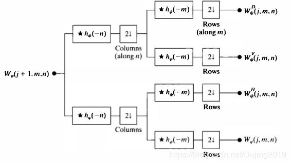
图7-3 The 2-D fast wavelet transform (FWT) filter bank
Each pass generates one DWT scale. In the first iteration, Wφ(j+ l.m.n) = f(x,y).
3.1.1 FWTs Using the Wavelet Toolbox
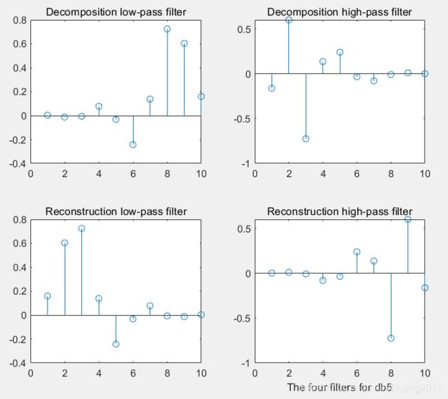
The Wavelet Toolbox provides decomposition filters for a wide variety of fast wavelet transforms. The filters associated with a specific transform are accessed via the function wfilters, which has the following general syntax:
[Lo_D, Hi_D, Lo_R, Hi_RJ = wfilters(wname)
[F1,F2] = wfilters(‘wname’,‘type’)
Refer to example 1 in the appendix for the experimental code
If type is set to 'd','r','l' or 'h', a pair of decomposition, reconstruction, low-pass and high-pass filters can be obtained, respectively.See table 7.1.If this syntax is called, the decomposition or low-pass filter will be returned in F1, with the result in F2.
Here are the four filters:
- Lo_D, the decomposition low-pass filter
- Hi_D, the decomposition high-pass filter
- Lo_R, the reconstruction low-pass filter
- Hi_R, the reconstruction high-pass filter
TABLE 7.1
| Lo_D and Hi_D |
(Decomposition filters) |
If ‘type’ = ‘d’ |
| Lo_R and Hi_R |
(Reconstruction filters) |
If ‘type’ = ‘r’ |
| Lo_D and Lo_R |
(Low-pass filters) |
If ‘type’ = ‘l’ |
| Hi_D and Hi_R |
(High-pass filters) |
If ‘type’ = ‘h’ |
TABLE 7.2 Wavelet Toolbox FWT filters and filter family names.
| Wavelet |
wfamily |
wname |
| Haar |
‘haar’ |
‘haar’ |
| Daubechies |
‘db’ |
‘db1’ or ‘haar’, ‘db2’, … ,‘db10’, … , ‘db45’ |
| Coiflets |
‘coif’ |
‘coif1’, … , ‘coif5’ |
| Symlets |
‘sym’ |
‘sym2’, … , ‘sym8’, … ,‘sym45’ |
| Discrete Meyer |
‘dmey’ |
‘dmey’ |
| Biorthogonal |
‘bior’ |
‘bior1.1’, ‘bior1.3’,… ‘bior6.8’ |
| Reverse Biorthogonal |
‘rbio’ |
‘rbio1.1’, ‘rbio1.3’, … ‘rbio6.8’ |
In order to print the description information of wfamily(see table 7-2) in the command window of MATLAB, enter it at the MALTAB prompt:
waveinfo(wfamily)
Refer to example 2 in the appendix for the experimental code
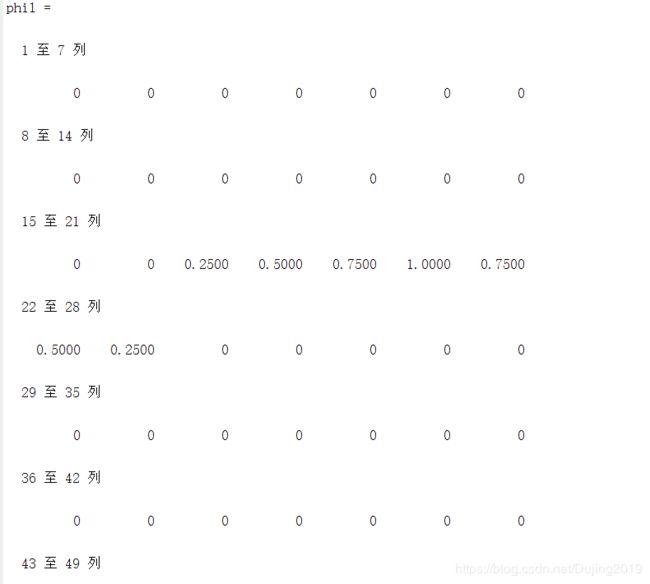
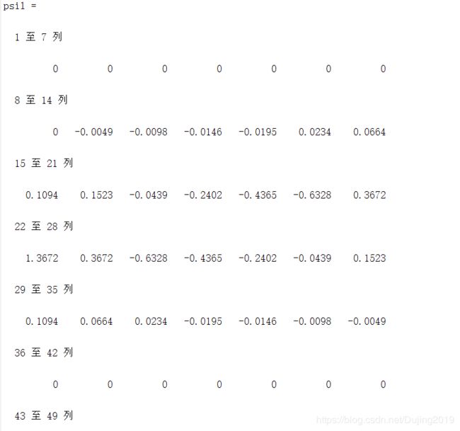
In order to obtain the scale of normalized orthogonal transformation and the numerical approximation of wavelet function, it can be typed as:
[phi, psi, xval] = wavefun(wname, iter)
Refer to example 3 in the appendix for the experimental code
Given a set of decomposition filters, whether user provided or generated by the wf il t e rs function, the simplest way of computing the associated wavelet transform is through the Wavelet Toolbox's wavedec2 function. It is invoked using :
[C,S] = wavedec2(X,N,Lo D,Hi D)
where Xis a 2-D image or matrix, N is the number of scales to be computed (i.e., the number of passes through the FWT filter bank in Fig. 7.2), and Lo_D and Hi_D are decomposition filters. The slightly more efficient syntax :
[C, S] = wavedec2(X, N, wname)
The experimental code refers to 4.1 and 4.2 of the experimental setup
To conclude this section, we note that because the FWT is based on digital filtering techniques and thus convolution, border distortions can arise. To minimize these distortions, the border must be treated differently from the other parts of the image. When filter elements fall outside the image during the convolution process, values must be assumed for the area, which is about the size of the filter, outside the image. Many Wavelet Toolbox functions, including the wavedec2 function, extend or pad the image being processed based on global parameter dwtmode. To examine the active extension mode, enter st = dwtmode ( 'status' ) or simply dwtmode at the MATLAB command prompt (e.g., > > dwtmode). To set the extension mode to STATUS, enter dwtmode(STATUS); to make STATUS the default extension mode, use dwtmode ( ' save' , STATUS). The supported extension modes and corresponding STATUS values are listed in Table 7.3.
TABLE 7.3 Wavelet Toolbox image extension or padding modes.
| STATUS |
Description |
| ‘sym’ |
The image is extended by mirror reflecting it across its borders. This is the normal default mode |
| 'zpd ’ |
The image is extended by padding with a value of 0. |
| ‘spd’ , 'sp1 ’ |
The image is extended by first-order derivative extrapolation-or padding with a linear extension of the outmost two border values. |
| 'spO ’ |
The image is extended by periodic padding. |
| 'ppd ’ |
The image is extended by mirror reflecting it across its borders. This is the normal default mode |
| ‘per’ |
Description The image is extended by mirror reflecting it across its borders. This is the normal default mode. The image is extended by padding with a value of 0. The image is extended by first-order derivative extrapolation-or padding with a linear extension of the outmost two border values. The image is extended by extrapolating the border values-that is, by boundary value replication. The image is extended by periodic padding. The image i extended by periodic padding after it has been padded (if necessary) to an even size using ‘spO’ extension. |
3.1.2 FWTs without the Wavelet Toolbox
In this section, we develop a pair of custom functions, wavefilter and wavefast, to replace the Wavelet Toolbox functions, wf il ters and wavedec2, of the previous section. Our goal is to provide additional insight into the mechanics of computing FWTs, and to begin the process of building a "standalone package" for wavelet-based image processing without the Wavelet Toolbox.
The first step is to devise a function for generating wavelet decomposition and reconstruction filters. The following function, which we call wavefilter, uses a standard switch construct, together with case and otherwise, to do this in a readily extendable manner.
function [varargout] = wavefilter(wname, type)
Refer to example 4 in the appendix for the function code
Note that for each orthonormal filter in wavefil ter (i.e., 'haar', 'db4 ', and ' sym4' ), the reconstruction filters are time-reversed versions of the decomposition filters and the highpass decomposition filter is a modulated version of its lowpass counterpart. Only the lowpass decomposition filter coefficients need to be explicitly enumerated in the code. The remaining filter coefficients can be computed from them. In wavef ilter, time reversal is carried out by reordering filter vector elements from last to first with statements like 1 r (end: -1 : 1 ) = ld. Modulation is accomplished by multiplying the components of a known filter by cos (pi *t), which alternates between 1 and -1 as t increases from 0 in integer steps. For each biorthogonal filter in wavefilter (i.e., 'bior6. 8' and ' jpeg9. 7 ' ), both the lowpass and highpass decomposition filters are specified; the reconstruction filters are computed as modulations of them. Finally, we note that the filters generated by wavefilter are of even length. Moreover, zero padding is used to ensure that the lengths of the decomposition and reconstruction filters of each wavelet are identical.
Given a pair of wavefilter generated decomposition filters, it is easy to write a general-purpose routine for the computation of the related FWT. The goal is to devise an efficient algorithm based on the filtering and downsampling operations in Fig. 7.3. To maintain compatibility with the existing Wavelet Toolbox, we employ the same decomposition structure (i.e., [ C, S] where C is a decomposition vector and S is a bookkeeping matrix). Because wavedec2 can accept M X N X 3 inputs, we also accept arrays that are extended along a third dimension. That is, the input can contain more than one 2-D array-like the red, green, and blue components of an RGB image. Each 2-D array of the extended array is called a page and its third index is called the page index. The following routine, which we call wavefast, uses symmetric image extension to reduce the border distortion associated with the computed FWT(s):
function [c, s] = wavefast(x, n, varargin)
function nc = addcoefs(c, x, pages)
function [y, keep] = symextend(x, fl, pages)
function y = symconv(x, h, type, fl, keep, pages)
Refer to example 5 in the appendix for the function code
As can be seen in the main routine, only one for loop, which cycles through the decomposition levels (or scales) that are generated, is used to orchestrate the entire forward transform computation. For each execution of the loop, the current approximation cell array app-whose elements are initially set to the 2-D images (or pages) of x-are symmetrically extended by internal function symextend. This function calls padarray, which was introduced in Section 3.4.2, to extend the matrices of app in two dimensions by mirror reflecting f1 - 1 of their elements (the length of the decomposition filter minus 1) across their borders.
Function symextend returns a cell array of extended approximation matrices and the number of pixels that should be extracted from the center of any subsequently convolved and downsampled results. The rows of the extended approximations are next convolved with highpass decomposition filter hp and downsampled via symconv. This function is described in the following paragraph. Convolved output, rows (also a cell array), is then submitted to symconv to convolve and downsample its columns with filters hp and lp-generating the diagonal and vertical detail coefficients of the top two branches of Fig. 7.3. These results are inserted into decomposition vector c by function addcoefs (working from the last element toward the first) and the process is repeated in accordance with Fig. 7.3 to generate the horizontal detail and approximation coefficients (the bottom two branches of the figure).
Function symconv uses the conv2 function to do the bulk of the transform computation work. It convolves filter h with the rows or columns of each matrix in cell array x (depending on type), discards the even indexed rows or columns (i.e., downsamples by 2), and extracts the center keep elements of each row or column. Invoking conv2 with cell array x and row filter vector h initiates a row-by-row convolution with each matrix in x; using column filter vector h' results in columnwise convolutions.
Compare the execution times of functions wavefast and wacedec2 in 4.3 of the experimental setup
3.2 Working with Wavelet Decomposition Structures
The wavelet transformation functions of the previous two sections generate nondisplayable data structures of the form {c, S}, where c is a transform coefficient vector and Sis a bookkeeping matrix that defines the arrangement of coefficients in c. To process images, we must be able to examine and/or modify c. In this section, we formally define {c, S}, examine some of the Wavelet Toolbox functions for manipulating it, and develop a set of custom functions that can be used without the Wavelet Toolbox. These functions are then used to build a general purpose routine for displaying c. The representation scheme introduced in Example 7.3 integrates the coefficients of a multiscale two-dimensional wavelet transform into a single,one-dimensional vector

where $A_N$ is the approximation coefficient matrix of the Nth decomposition level and Hi, Vi, and Di for i = 1, 2, ... N are the horizontal, vertical, and diagonal transform coefficient matrices for level i. Here, Hi( : )' for example, is the row vector formed by concatenating the transposed columns of matrix Hi.That is ,if

Then


Because the equation for c assumes N decompositions (or passes through the filter bank in Fig. 7.3), c contains 3N + 1 sections-one approximation and N groups of horizontal, vertical, and diagonal details. Note that the highest scale coefficients are computed when i = l; the lowest scale coefficients are associated with i = N. Thus, the coefficients of care ordered from low to high scale.
Wavelet Toolbox functions for manipulating transform decomposition vector c in example 4 of the experimental setup.
3.2.1 Editing Wavelet Decomposition Coefficients without the Wavelet Toolbox
Without the Wavelet Toolbox, bookkeeping matrix S is the key to accessing the individual approximation and detail coefficients of multiscale vector c. In this section, we use S to build a set of general-purpose routines for the manipulation of c. Function wavework is the foundation of the routines developed, which are based on the familiar cut-copy-paste metaphor of modern word processing applications.
function [varargout] = wavework(opcode, type, c, s, n, x)
Refer to example 6 in the appendix for the function code
As wavework checks its input arguments for reasonableness, the number of elements in each coefficient submatrix of c is computed via elements = prod(s, 2). MATLAB function Y = prod(X, DIM) computes the products of the elements of X along dimension DIM. The first switch statement then begins the computation of a pair of pointers to the coefficients associated with input parameters type and n. For the approximation case, the computation is trivial since the coefficients are always at the start of c (i.e., start is 1); the ending index is of course the number of elements in the approximation matrix, which is elements ( 1). When a detail coefficient submatrix is requested, however, start is computed by summing the number of elements at all decomposition levels above n and adding offset * elements ( nindex); where offset is 0, 1, or 2 for the horizontal, vertical, or diagonal coefficients, respectively, and nindex is a pointer to the row of s that corresponds to input parameter n.
The second switch statement in function wavework performs the operation requested by opcode. For the 'cut' and 'copy' cases, the coefficients of c between start and stop are copied into vector y, which is then "reshaped" to create a 2-D matrix whose size is determined by s. This is done using y = reshape ( y, s ( nindex, : ) ) , where the generalized MATLAB function :
y = reshape(x,m,n)
returns an m by n matrix whose elements are taken column wise from x. An error is returned if x does not have m*n elements. For the 'paste' case, the elements of x are copied into c between start and stop. For both the 'cut' and 'paste' operations, a new decomposition vector nc is returned.
The following three functions-wavecut, wavecopy, and wavepaste-use wavewo rk to manipulate c using a more intuitive syntax:
function [nc, y] = wavecut(type, c, s, n)
function y = wavecopy(type, c, s, n)
function nc = wavepaste(type, c, s, n, x)
Refer to example 7 in the appendix for the function code
Using function wavecut and function wavecopy to process c in 4. 4 of the experimental setup
3.2.2 Displaying Wavelet Decomposition Coefficients
In reality, the coefficients of the two-dimensional output arrays from the filter bank in Fig. 7.3. For each iteration of the filter bank, four quarter-size coefficient arrays (neglecting any expansion that may result from the convolution process) are produced. They can be arranged as a 2 X 2 array of submatrices that replace the twodimensional input from which they are derived. Function **wavedisplay** performs a similar subimage compositing; it scales the coefficients to better reveal their differences and inserts borders to delineate the approximation and various horizontal, vertical, and diagonal detail matrices.
function w = wavedisplay(c, s, scale, border)
Refer to example 8 in the appendix for the function code
The subimage in the upper left corner of w, for instance, is the approximation array that results from the final decomposition step. It is surrounded-in a clockwise manner-by the horizontal, diagonal, and vertical detail coefficients that were generated during the same decomposition. The resulting array of subimages is then surrounded (again in a clockwise manner) by the detail coefficients of the previous decomposition step; and the pattern continues until all of the scales of decomposition vector c are appended to two-dimensional matrix w.
Using function wavedisplay to display conversion coefficient in 4.5 of the experimental setup
3.3 The Inverse Fast Wavelet Transform
Like its forward counterpart, the inverse fast wavelet transform can be computed iteratively using digital filters. Figure 8.6 shows the required synthesis or reconstruction filter bank, which reverses the process of the analysis or decomposition filter bank of Fig. 8.2. At each iteration, four scale j approximation and detail subimages are upsampled (by inserting zeroes between every other element) and convolved with two one-dimension filters-one operating on the subimages' columns and the other on its rows. Addition of the results yields the scale j + 1 approximation, and the process is repeated until the original image is reconstructed. The filters used in the convolutions are a function of the wavelets employed in the forward transform.

FIGURE 7.4
When using the Wavelet Toolbox, function waverec2 is employed to compute the inverse FWT of wavelet decomposition structure [ C, S]. It is invoked using
g = waverec2(C, S, wname)
where g is the resulting reconstructed two-dimensional image (of class double). The required reconstruction filters can be alternately supplied via syntax :
g = waverec2(C, S, Lo_R, Hi_R)
The following custom routine, which we call waveback, can be used when the Wavelet Toolbox is unavailable. It is the final function needed to complete our wavelet-based package for processing images in conjunction with the Image Processing Toolbox (and without the Wavelet Toolbox).
function [varargout] = waveback(c, s, varargin)
Refer to example 9 in the appendix for the function code
The main routine of function waveback is a simple for loop that iterates through the requested number of decomposition levels (i.e., scales) in the desired reconstruction. As can be seen, each loop calls internal function symco nvup four times and sums the returned matrices. Decomposition vector nc, which is initially set to c, is iteratively updated by replacing the four coefficient matrices passed to symconvup by the newly created approximation a. Bookkeeping matrix ns is then modified accordingly-there is now one less scale in decomposition structure [ nc, ns]. This sequence of operations is slightly different than the ones outlined in Fig. 7.4, in which the top two inputs are combined to yield :

Function waveback uses the equivalent computation :

Function symconvup performs the convolutions and upsampling required to compute the contribution of one input of Fig. 8.6 to output W φ
Compare the execution times of functions waverec2 and waveback in 4.7 of the experimental setup
3.4 Wavelets in Image Processing
As in the Fourier domain, the basic approach to waveletbased image processing is to
1. Compute the two-dimensional wavelet transform of an image.
2. Alter the transform coefficients.
3. Compute the inverse transform.
This section mainly studies the orientation and edge detection of wavelet, image smoothing and blurring based on wavelet, and progressive reconstruction. For specific experimental steps, please refer to 4.8, 4.9 and 4.10 of the experimental setup.
4. Experimental Setup
In this section, 10 experiments on wavelets are illustrated.Among them are wavelet transform function, sensitivity and edge detection of two-dimensional wavelet transform direction, image smoothing and blurring based on wavelet, and progressive reconstruction, etc. Wavelet transform and its application in image processing are introduced.
4.1 Haar filters, scaling, and wavelet functions.
The oldest and simplest wavelet transform is based on the Haar scaling and wavelet functions. The decomposition and reconstruction filters for a Haar-based transform are of length 2 and can be obtained as follows:
[Lo_D, Hi_D, Lo_R, Hi_R] = wfilters( 'haar')
The code operation effect is as follows:

Their key properties (as reported by the wave info function) and plots of the associated scaling and wavelet functions can be obtained using :
waveinfo( 'haar');

 [phi, psi, xval] = wavefun( 'haar', 10);
 xaxis = zeros(size(xval));
 subplot(1,2,1);
 plot(xval, phi, 'k', xval, xaxis, '--k');
 axis([0 1 -1.5 1.5]); axis square;
 title('Haar Scaling Function');
 subplot(1,2,2); plot(xval, psi, 'k', xval, xaxis, '--k');
 axis([0 1 -1.5 1.5]); axis square;
 title('Haar Wavelet Function');
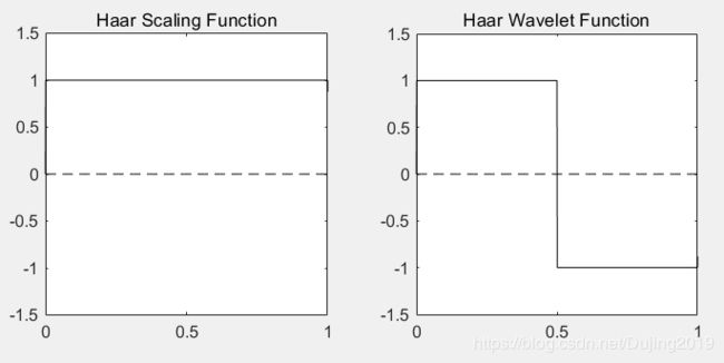
FIGURE 7.5 Haar scaling and wavelet functions.
The Haar scaling and wavelet functions shown in Fig. 7.3 are discontinuous and compactly supported, which means they are 0 outside a finite interval called the support. Note that the support is 1. In addition, the waveinfo data reveals that the Haar expansion functions are orthogonal, so that the forward and inverse transformation kernels are identical.
4.2 A simple FWT using Haar filters.
Consider the following single-scale wavelet transform with respect to Haar wavelets:
f = magic(4);

[c1,s1]=wavedec2(f,1,'haar')
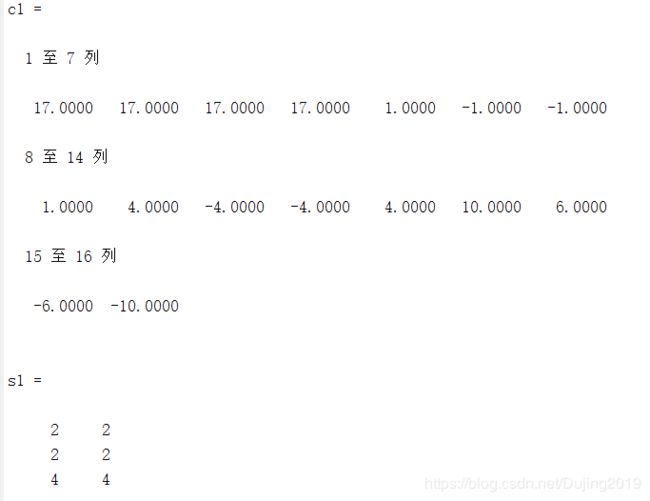
Here, a 4 x 4 magic square f is transformed into a 1x16 wavelet decomposition vector c1 and 3 X 2 bookkeeping matrix s 1. The entire transformation is performed with a single execution (with f used as the input) of the operations depicted in Fig. 7.3. Four 2 X 2 outputs-a downsampled approximation and three directional (horizontal, vertical, and diagonal) detail matrices-are generated. Function wavedec2 concatenates these 2 X 2 matrices columnwise in row vector c1 beginning with the approximation coefficients and continuing with the horizontal, vertical, and diagonal details. That is, c1 (1) through c1 (4) are approximation coefficients Wφ(l,0,0), Wφ(l, 1,0), Wφ(l,O, 1), and Wφ(l, 1, 1) from Fig. 7.3 with the scale of f assumed arbitrarily to be 2; c1 (5) through c1 (8) are $w_Ψ$H(l,O,O), $w_Ψ$H(l,l,O), $w_Ψ$H(l,O,l), and $w_Ψ$H(1,1,1); and so on. It we were to extract the horizontal detail coefficient matrix from vector c1, for example, we would get

When the single-scale transform described above is extended to two scales, we get
[c2, s2] = wavedec2(f, 2, 'haar')
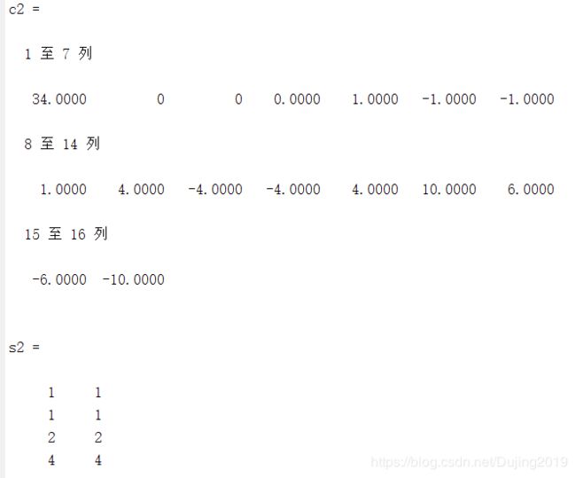
Note that c2(5:16) = c1 (5:16). Elements c1 (1 :4), which were the approximation coefficients of the single-scale transform, have been fed into the filter bank of Fig. 8.2 to produce four 1X1 outputs: Wφ(O, 0, 0), $w_Ψ$H (0, 0, 0), $w_Ψ$V(0, 0, 0), and $w_Ψ$D(0 , 0, 0). These outputs are concatenated columnwise (though they are lX 1 matrices here) in the same order that was used in the preceding single-scale transform and substituted for the approximation coefficients from which they were derived. Bookkeeping matrix s2 is then updated to reflect the fact that the single 2 X 2 approximation matrix in c1 has been replaced by four 1 x 1 detail and approximation matrices in c2. Thus, s2 (end, : ) is once again the size of the original image, s2 ( 3, : ) is the size of the three detail coefficient matrices at scale 1, s2 ( 2, : ) is the size of the three detail coefficient matrices at scale 0, and s2 ( 1 , : ) is the size of the final approximation.
4.3 Comparing the execution times ofwavefast and wavedec2.
The following test routine uses function time it from Chapter 2 to compare the execution times of the Wavelet Toolbox function wavedec2 and custom function wavefast:
function [ratio, maxdiff] = fwtcompare(f, n, wname)

% Get transform and computation time for wavedec2.
w1 = @() wavedec2(f, n, wname);
reftime = timeit(w1);

% Get transform and computation time for wavefast.
w2 = @() wavefast(f, n, wname);
t2 = timeit(w2);

% Compare the results.
ratio = t2 / reftime;
maxdiff = abs(max(w1() - w2()));
f = imread('D:\Dip\Chapter7\sun.jpg');
[ratio, maxdifference] = fwtcompare(f, 5, 'db4')

Note that custom function wavefast was faster than its Wavelet Toolbox counterpart while producing virtually identical results.
4.4 Wavelet Toolbox functions for manipulating transform decomposition vector c.
The Wavelet Toolbox provides a variety of functions for locating, extracting, reformatting, and/or manipulating the approximation and horizontal, vertical, and diagonal coefficients of c as a function of decomposition level. We introduce them here to illustrate the concepts just discussed and to prepare the way for the alternative functions that will be developed in the section.Consider,for example,the following sequence of commands:
f = magic(8);
[c1,s1]=wavedec2(f,3,'haar');
approx = appcoef2(c1,s1,'haar');
horizdet2 = detcoef2( 'h', c1 , s1, 2);
newc1 = wthcoef2('h', c1 , s1, 2);
newhorizdet2 = detcoef2('h', newc1 , s1 , 2)
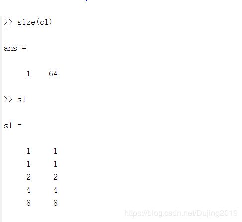
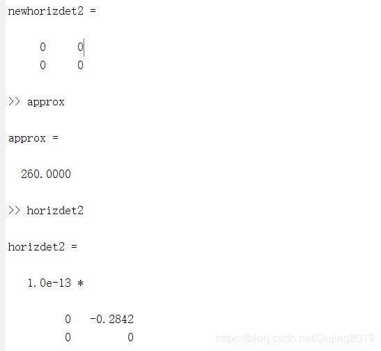
Here, K is 1 and a three-level decomposition with respect to Haar wavelets is performed on a single 8 x 8 magic square using the wavedec function. The resulting coefficient vector, c 1, is of size 1 X 64. Since s 1 is 5 x 2 we know that the coefficients of c1 span (N -2) = (5 -2) = 3 decomposition levels. Thus. it concatenates the elements needed to populate 3N + 1 = 3(3) + 1 = 10 approximation and detail coefficient submatrices. Based on s1, these submatrices include (a) a 1X1 approximation matrix and three 1 X 1 detail matrices for decomposition level 3 [see s 1 ( 1 , : ) and s 1 ( 2, : ) ], (b) three 2 X 2 detail matrices for level 2 [see s1 (3, : )], and (c) three 4X4 detail matrices for level 1 [see s 1 ( 4, : ) ). The fifth row of s 1 contains the size of the original image f.
4.5 Manipulating c with wavecut and wavecopy.
Functions wavecopy and wavecut can be used to reproduce the Wavelet Toolbox based results of Example 4.4:
f = magic(8);
[c1,s1]=wavedec2(f,3,'haar');
approx = wavecopy('a',c1,s1);
horizdet2 = wavecopy( 'h', c1 , s1, 2);
[newc1,horizdet2] = wavecut('h', c1 , s1, 2);
newhorizdet2 = wavecopy('h', newc1 , s1 , 2)
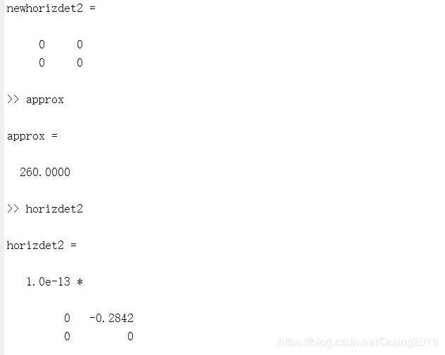
Note that all extracted matrices are identical to those of the previous .
4.6 Transform coefficient display using wavedisplay.
The following sequence of commands computes the two-scale DWT of the image in Fig. 7.5 with respect to fourth-order Daubechies' wavelets and displays the resulting coefficients:
f = imread('D:\Dip\Chapter7\Fig0704.tif');
[c,s] = wavefast(f, 2, 'db4');title('(a) Automatic scaling; ');
wavedisplay(c, s); title('(a) Automatic scaling; ');
figure; wavedisplay(c, s, 8);title('(b) additional scaling by 8; ');
figure; wavedisplay(c, s,-8) ; title('(c) absolute values scaled by 8. ');
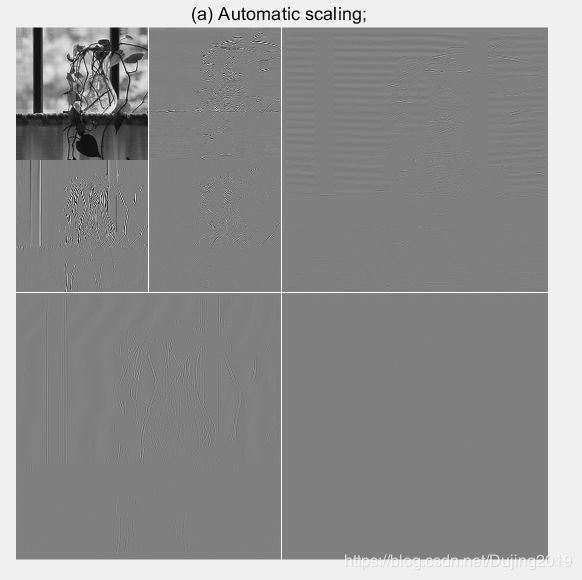
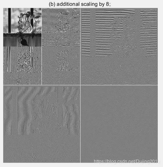
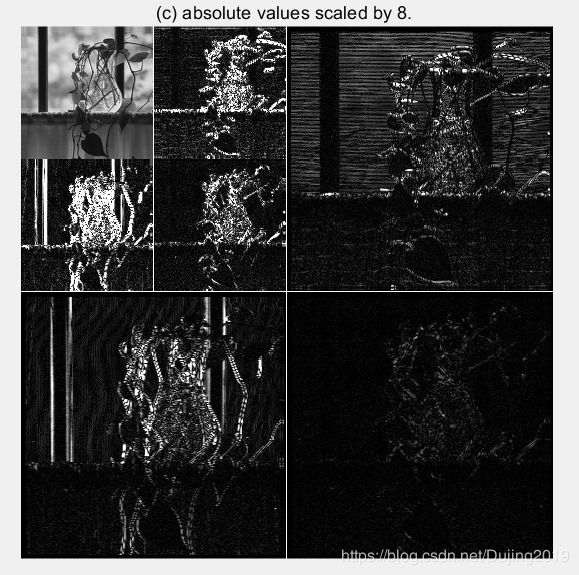
FIGURE 7.5
The images generated by the final three command lines are shown in ( a) through (c), respectively. Without additional scaling, the detail coefficient differences in (a) are barely visible. In (b ), the differences are accentuated by multiplying the coefficients by 8. Note the mid-gray padding along dimensional variations between transform coefficient subimages. Figure (c) shows the effect .
4.7 Comparing the execution times of waveback and waverec2.
The following test routine compares the execution times of Wavelet Toolbox function waverec2 and custom function waveback using a simple modification of the test function in Example 4.3:
function [ratio, maxdiff] = ifwtcompare(f, n, wname)
[c1, s1] = wavedec2(f, n, wname);
w1 = @() waverec2(c1, s1, wname);
reftime = timeit(w1);

% Compute the transform and get output and computation time for
% waveback.
[c2, s2] = wavefast(f, n, wname);
w2 = @() waveback(c2, s2, wname);
t2 = timeit(w2);

% Compare the results.
ratio = t2 / reftime;
diff = double(w1()) - w2();
maxdiff = abs(max(diff(:)));
f = imread('D:\Dip\Chapter7\sun.jpg');
[ratio, maxdifference] = ifwtcompare(f, 5, 'db4');

Note that the inverse transformation times of the two functions are similar (i.e., the ratio is 1.2238) and that the largest output difference is 3.6948X10(-13). For all practical purposes, they essentially equivalent.
4.8 Wavelet directionality and edge detection.
Here, we use a image to demonstrate the directional sensitivity of the 2-D wavelet transform and its usefulness in edge detection:
f = imread('D:\Dip\Chapter7\Fig0707(a).tif');
subplot(2, 2, 1);imshow(f); title('(a) A simple test image;');
[c, s] = wavefast(f, 1, 'sym4');
subplot(2, 2, 2); imshow(wavedisplay(c, s, -6)) ; title('(b) its wavelet transform;');
[ nc, y] = wavecut ( 'a' , c, s) ;
subplot(2, 2, 3); imshow(wavedisplay(nc, s, -6)) ; title('(c) the transform modified by zeroing all approximation coefficients;');
edges = abs (waveback ( nc, s, 'sym4' ) ) ;
subplot(2, 2, 4); imshow(mat2gray(edges)); title('( d) the edge image resulting from computing the absolute value of the inverse transform.');
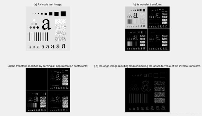
FIGURE 7.6
The horizontal, vertical, and diagonal directionality of the single-scale wavelet transform of Fig.(a) with respect to ' sym4 ' wavelets is clearly visible in Fig. (b ). Note, for example, that the horizontal edges of the original image are present in the horizontal detail coefficients of the upper-right quad rant of Fig. (b ). The vertical edges of the image can be similarly identified in the vertical detail coefficients of the lower-left quadrant. To combine this information into a single edge image, we simply zero the approximation coefficients of the generated transform, compute its inverse, and take the absolute value. The modified transform and resulting edge image are shown in Figs. (c) and (d), respectively. A similar procedure can be used to isolate the vertical or horizontal edges alone.
4.9 Wavelet-based image smoothing or blurring.
Wavelets, like their Fourier counterparts, are effective instruments for smoothing or blurring images. Consider again the test image of Fig. 7.6(a), which is repeated in Fig. 7.7(a). Its wavelet transform with respect to fourthorder symlets is shown in Fig. 7.7(b ), where it is clear that a four-scale decomposition has been performed. To streamline the smoothing process, we employ the following utility function:
f = imread('D:\Dip\Chapter7\Fig0707(a).tif');
figure;imshow(f);title('(a)the original image');
[c, s] = wavefast(f, 4, 'sym4');   %Fast wavelet decomposition is performed on scale 4
figure;
wavedisplay(c, s, 20) ;   %Reconstruction on 20 scales
title('(b)sym4 four wavelet transform results');
[c,g8] = wavezero(c, s,1,'sym4'); %This function will automatically draw a window and set the size detail to 0
title('(c)Set the details of scale 1 to 0 after the inverse transformation');
[c, g8] = wavezero(c, s, 2, 'sym4');
title('(d)Set the details of scale 2 to 0 after the inverse transformation');
[c, g8] = wavezero(c, s, 3, 'sym4');
title('(e)Set the details of scale 3 to 0 after the inverse transformation');
[c, g8] = wavezero(c, s, 4, 'sym4');
title('(f)Set the details of scale 4 to 0 after the inverse transformation');
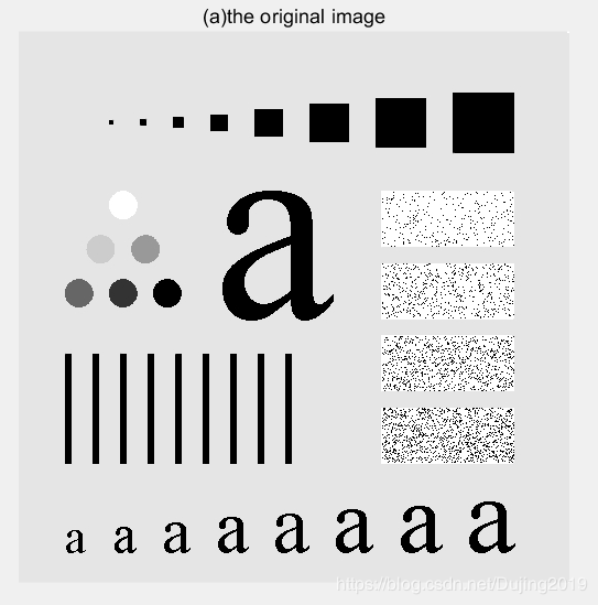
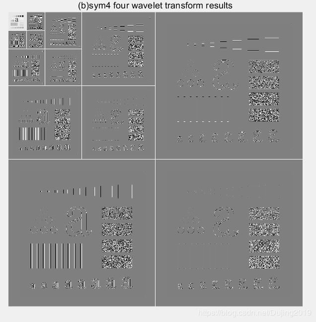

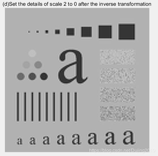

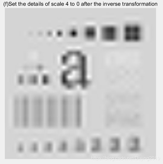
FIGURE 7.7 Wavelet-based image smoothing
Note that the smoothed image in Fig. 7.7(c) is only slightly blurred, as it was obtained by zeroing only the first-level detail coefficients of the original image's wavelet transform (and computing the modified transform 's inverse). Additional blurring is present in the second result-Fig. 7.7(d)-which shows the effect of zeroing the second level detail coefficients as well. The coefficient zeroing process continues in Fig. 7.7( e ), where the third level of details is zeroed, and concludes with Fig. 7.7(f), where all the detail coefficients have been eliminated. The gradual increase in blurring from Figs. 7.7( c) to (f) is reminiscent of similar results with Fourier transforms. It illustrates the intimate relationship between sca le in the wavelet domain and frequency in the Fourier domain.
4.10 Progressive reconstruction.
Consider next the transmission and reconstruction of the four-scale wavelet transform in Fig. 7.8(a) within the context of browsing a remote image database for a specific image. Here, we deviate from the three-step procedure described at the beginning of this section and consider an application without a Fourier domain counterpart.
f = rgb2gray(imread('D:\Dip\Chapter7\sun.jpg'));
%figure;imshow(f);title('(d)the original image');
figure;[c, s] = wavefast(f, 4, 'jpeg9.7');   %4 Scale wavelet decomposition
wavedisplay(c,s,8);   %Reconstruction on 20 scales
title('(a)4 scaling wavelet decomposition coefficient (reconstruction)');
f=wavecopy('a',c,s);%Wavelet decomposition myopia coefficient matrix is obtained
figure,imshow(mat2gray(f));
title('(b)Wavelet image of myopia coefficient');
[c s]=waveback(c,s,'jpeg9.7',1);
f=wavecopy('a',c,s);
figure,imshow(mat2gray(f));%The reconstructed myopic wavelet coefficient image
title('(c)The image was reconstructed 1 time');
[c s]=waveback(c,s,'jpeg9.7',1);
f=wavecopy('a',c,s);
figure,imshow(mat2gray(f));%The reconstructed myopic wavelet coefficient image
title('(d)The image was reconstructed twice');
[c s]=waveback(c,s,'jpeg9.7',1);
f=wavecopy('a',c,s);
figure,imshow(mat2gray(f));%The reconstructed myopic wavelet coefficient image
title('(e)The image was reconstructed 3 times');
[c s]=waveback(c,s,'jpeg9.7',1);
f=wavecopy('a',c,s);
figure,imshow(mat2gray(f));%The reconstructed myopic wavelet coefficient image
title('(f)The image was reconstructed 4 times');

FIGURE 7.8
Each image in the database is stored as a multiscale wavelet decomposition. This structure is well suited to progressive reconstruction applications, particularly when the 1-D decomposition vector used to store the transform 's coefficients assumes the general format of Section 3.2. For the four-scale transform of this example, the decomposition vector is

where A4 is the approximation coefficient matrix of the fourth decomposition level and Hi, Vi, and Di for i = 1, 2, 3, 4 are the horizontal, vertical, and diagonal transform coefficient matrices for level i. If we transmit this vector in a left-to-right manner, a remote display device can gradually build higher resolution approximations of the final high-resolution image (based on the user's needs) as the data arrives at the viewing station. For instance, when the A4 coefficients have been received, a low-resolution version of the image can be made available for viewing [Fig. 7.8(b)]. When H4, V4, and D4 have been received, a higher-resolution approximation [Fig. 7.8( c)] can be constructed, and so on. Figures 7.8(d) through (f) provide three additional reconstructions of increasing resolution. Note that the final four approximations use waveback to perform single level reconstructions.
5. Conclusion
The material in this chapter introduces the wavelet transform and its use in image processing. Like the Fourier transform, wavelet transforms can be used in tasks ranging from edge detection to image smoothing, both of which are considered in the material that is covered. Because they provide significant insight into both an image's spatial and frequency characteristics, wavelets can also be used in applications in which Fourier methods are not well suited, like progressive image reconstruction (see Example 7.10). Because the Image Processing Toolbox does not include routines for computing or using wavelet transforms, a significant portion of this chapter is devoted to the development of a set of functions that extend the Image Processing Toolkit to wavelet-based imaging. The functions developed were designed to be fully compatible with MATLAB's Wavelet Toolbox, which is introduced in this chapter but is not a part of the Image Processing Toolbox.
6. Appendix
Example 1:
Write the code:
% Set the name of the wavelet
wname = 'db5';
%wname = 'bior2.6';
%wname = 'rbio2.6';

% Calculate four filters for a given wavelet

[Lo_D,Hi_D,Lo_R,Hi_R] = wfilters(wname);
subplot(221); stem(Lo_D);
title('Decomposition low-pass filter');
subplot(222); stem(Hi_D);
title('Decomposition high-pass filter');
subplot(223); stem(Lo_R);
title('Reconstruction low-pass filter');
subplot(224); stem(Hi_R);
title('Reconstruction high-pass filter');
xlabel('The four filters for db5')
The code operation effect is as follows:


Example 2
Write the code:
wfamily = 'haar';
waveinfo(wfamily);
The code operation effect is as follows:

Example 3
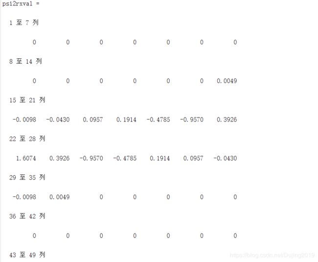
Write the code::
wname = 'rbio2.6';
[phil,psil,phi2,psi2rxval] = wavefun(wname,2)
The code operation effect is as follows:

Example 4
function [varargout] = wavefilter(wname, type)
% Check the input and output arguments.
error(nargchk(1, 2, nargin));

if (nargin == 1 && nargout ~= 4) || (nargin == 2 && nargout ~= 2)
   error('Invalid number of output arguments.');
end

if nargin == 1 && ~ischar(wname)
   error('WNAME must be a string.');
end

if nargin == 2 && ~ischar(type)
   error('TYPE must be a string.');
end

% Create filters for the requested wavelet.
switch lower(wname)
case {'haar', 'db1'}
   ld = [1 1]/sqrt(2);     hd = [-1 1]/sqrt(2);
   lr = ld;                hr = -hd;

case 'db4'
   ld = [-1.059740178499728e-002 3.288301166698295e-002 ...
         3.084138183598697e-002 -1.870348117188811e-001 ...
         -2.798376941698385e-002 6.308807679295904e-001 ...
         7.148465705525415e-001 2.303778133088552e-001];
   t = (0:7);
   hd = ld;    hd(end:-1:1) = cos(pi * t) .* ld;
   lr = ld;    lr(end:-1:1) = ld;
   hr = cos(pi * t) .* ld;

case 'sym4'
   ld = [-7.576571478927333e-002 -2.963552764599851e-002 ...
         4.976186676320155e-001 8.037387518059161e-001 ...
         2.978577956052774e-001 -9.921954357684722e-002 ...
         -1.260396726203783e-002 3.222310060404270e-002];
   t = (0:7);
   hd = ld;    hd(end:-1:1) = cos(pi * t) .* ld;
   lr = ld;    lr(end:-1:1) = ld;
   hr = cos(pi * t) .* ld;

case 'bior6.8'
   ld = [0 1.908831736481291e-003 -1.914286129088767e-003 ...
         -1.699063986760234e-002 1.193456527972926e-002 ...
         4.973290349094079e-002 -7.726317316720414e-002 ...
         -9.405920349573646e-002 4.207962846098268e-001 ...
         8.259229974584023e-001 4.207962846098268e-001 ...
         -9.405920349573646e-002 -7.726317316720414e-002 ...
         4.973290349094079e-002 1.193456527972926e-002 ...
         -1.699063986760234e-002 -1.914286129088767e-003 ...
         1.908831736481291e-003];
   hd = [0 0 0 1.442628250562444e-002 -1.446750489679015e-002 ...
         -7.872200106262882e-002 4.036797903033992e-002 ...
         4.178491091502746e-001 -7.589077294536542e-001 ...
         4.178491091502746e-001 4.036797903033992e-002 ...
         -7.872200106262882e-002 -1.446750489679015e-002 ...
         1.442628250562444e-002 0 0 0 0];
   t = (0:17);
   lr = cos(pi * (t + 1)) .* hd;
   hr = cos(pi * t) .* ld;

case 'jpeg9.7'
   ld = [0 0.02674875741080976 -0.01686411844287495 ...
         -0.07822326652898785 0.2668641184428723 ...
         0.6029490182363579 0.2668641184428723 ...
         -0.07822326652898785 -0.01686411844287495 ...
         0.02674875741080976];
   hd = [0 -0.09127176311424948 0.05754352622849957 ...
         0.5912717631142470 -1.115087052456994 ...
         0.5912717631142470 0.05754352622849957 ...
         -0.09127176311424948 0 0];
   t = (0:9);
   lr = cos(pi * (t + 1)) .* hd;
   hr = cos(pi * t) .* ld;

otherwise
   error('Unrecognizable wavelet name (WNAME).');
end

% Output the requested filters.
if (nargin == 1)
   varargout(1:4) = {ld, hd, lr, hr};
else
   switch lower(type(1))
   case 'd'
      varargout = {ld, hd};
   case 'r'
      varargout = {lr, hr};
   otherwise
      error('Unrecognizable filter TYPE.');
   end
end
Example 5
function [c, s] = wavefast(x, n, varargin)
error(nargchk(3, 4, nargin));

if nargin == 3
   if ischar(varargin{1})
      [lp, hp] = wavefilter(varargin{1}, 'd');
   else
      error('Missing wavelet name.');
   end
else
   lp = varargin{1};   hp = varargin{2};
end

% Get the filter length, 'lp', input array size, 'sx', and number of
% pages, 'pages', in extended 2-D array x.
fl = length(lp);       sx = size(x);        pages = size(x, 3);

if ((ndims(x) ~= 2) && (ndims(x) ~= 3)) || (min(sx) < 2) ...
        || ~isreal(x) || ~isnumeric(x)
   error('X must be a real, numeric 2-D or 3-D matrix.');
end

if (ndims(lp) ~= 2) || ~isreal(lp) || ~isnumeric(lp) ...
       || (ndims(hp) ~= 2) || ~isreal(hp) || ~isnumeric(hp) ...
       || (fl ~= length(hp)) || rem(fl, 2) ~= 0
   error(['LP and HP must be even and equal length real, ' ...
          'numeric filter vectors.']);
end

if ~isreal(n) || ~isnumeric(n) || (n < 1) || (n > log2(max(sx)))
   error(['N must be a real scalar between 1 and ' ...
          'log2(max(size((X))).']);
end

% Init the starting output data structures and initial approximation.
c = [];        s = sx(1:2);
app = cell(pages, 1);
for i = 1:pages
   app{i} = double(x(:, :, i));
end

% For each decomposition ...
for i = 1:n
   % Extend the approximation symmetrically.
   [app, keep] = symextend(app, fl, pages);

   % Convolve rows with HP and downsample. Then convolve columns
   % with HP and LP to get the diagonal and vertical coefficients.
   rows = symconv(app, hp, 'row', fl, keep, pages);
   coefs = symconv(rows, hp, 'col', fl, keep, pages);
   c = addcoefs(c, coefs, pages);
   s = [size(coefs{1}); s];
   coefs = symconv(rows, lp, 'col', fl, keep, pages);
   c = addcoefs(c, coefs, pages);

   % Convolve rows with LP and downsample. Then convolve columns
   % with HP and LP to get the horizontal and next approximation
   % coeffcients.
   rows = symconv(app, lp, 'row', fl, keep, pages);
   coefs = symconv(rows, hp, 'col', fl, keep, pages);
   c = addcoefs(c, coefs, pages);
   app = symconv(rows, lp, 'col', fl, keep, pages);
end

% Append the final approximation structures.
c = addcoefs(c, app, pages);
s = [size(app{1}); s];
if ndims(x) > 2
   s(:, 3) = size(x, 3);
end

%-------------------------------------------------------------------%
function nc = addcoefs(c, x, pages)
% Add 'pages' array coefficients to the wavelet decomposition vector.

nc = c;
for i = pages:-1:1
   nc = [x{i}(:)' nc];
end

%-------------------------------------------------------------------%
function [y, keep] = symextend(x, fl, pages)
% Compute the number of coefficients to keep after convolution and
% downsampling. Then extend the 'pages' arrays of x in both
% dimensions.

y = cell(pages, 1);
for i = 1:pages
   keep = floor((fl + size(x{i}) - 1) / 2);
   y{i} = padarray(x{i}, [(fl - 1) (fl - 1)], 'symmetric', 'both');
end

%-------------------------------------------------------------------%
function y = symconv(x, h, type, fl, keep, pages)
% For the 'pages' 2-D arrays in x, convolve the rows or columns with
% h, downsample, and extract the center section since symmetrically
% extended.

y = cell(pages, 1);
for i = 1:pages
   if strcmp(type, 'row')
       y{i} = conv2(x{i}, h);
       y{i} = y{i}(:, 1:2:end);
       y{i} = y{i}(:, fl / 2 + 1:fl / 2 + keep(2));
   else
       y{i} = conv2(x{i}, h');
       y{i} = y{i}(1:2:end, :);
       y{i} = y{i}(fl / 2 + 1:fl / 2 + keep(1), :);
   end
end
Example 6
function [varargout] = wavework(opcode, type, c, s, n, x)
error(nargchk(4, 6, nargin));

if (ndims(c) ~= 2) || (size(c, 1) ~= 1)
   error('C must be a row vector.');
end

if (ndims(s) ~= 2) || ~isreal(s) || ~isnumeric(s) || ...
        ((size(s, 2) ~= 2) && (size(s, 2) ~= 3))
   error('S must be a real, numeric two- or three-column array.');
end

elements = prod(s, 2);                % Coefficient matrix elements.
if (length(c) < elements(end)) || ...
      ~(elements(1) + 3 * sum(elements(2:end - 1)) >= elements(end))
    error(['[C S] must form a standard wavelet decomposition ' ...
           'structure.']);
end

if strcmpi(opcode(1:3), 'pas') && nargin < 6
   error('Not enough input arguments.');
end

if nargin < 5
   n = 1;                        % Default level is 1.
end
nmax = size(s, 1) - 2;           % Maximum levels in [C, S].

aflag = (lower(type(1)) == 'a');
if ~aflag && (n > nmax)
   error('N exceeds the decompositions in [C, S].');
end

switch lower(type(1))            % Make pointers into C.
case 'a'
   nindex = 1;
   start = 1;    stop = elements(1);    ntst = nmax;
case  {'h', 'v', 'd'}
   switch type
   case 'h', offset = 0;         % Offset to details.
   case 'v', offset = 1;
   case 'd', offset = 2;
   end
   nindex = size(s, 1) - n;      % Index to detail info.
   start = elements(1) + 3 * sum(elements(2:nmax - n + 1)) + ...
           offset * elements(nindex) + 1;
   stop = start + elements(nindex) - 1;
   ntst = n;
otherwise
   error('TYPE must begin with "a", "h", "v", or "d".');
end

switch lower(opcode)             % Do requested action.
case {'copy', 'cut'}
   y = c(start:stop);    nc = c;
   y = reshape(y, s(nindex, :));
   if strcmpi(opcode(1:3), 'cut')
      nc(start: stop) = 0; varargout = {nc, y};
   else
      varargout = {y};
   end
case 'paste'
   if numel(x) ~= elements(end - ntst)
      error('X is not sized for the requested paste.');
   else
      nc = c;   nc(start:stop) = x(:);   varargout = {nc};
   end
otherwise
   error('Unrecognized OPCODE.');
end
Example 7
function [nc, y] = wavecut(type, c, s, n)
error(nargchk(3, 4, nargin));
if nargin == 4
   [nc, y] = wavework('cut', type, c, s, n);
else
   [nc, y] = wavework('cut', type, c, s);
end

function y = wavecopy(type, c, s, n)
error(nargchk(3, 4, nargin));
if nargin == 4
   y = wavework('copy', type, c, s, n);
else
   y = wavework('copy', type, c, s);
end

function nc = wavepaste(type, c, s, n, x)
error(nargchk(5, 5, nargin))
nc = wavework('paste', type, c, s, n, x);
Example 8
function w = wavedisplay(c, s, scale, border)
error(nargchk(2, 4, nargin));

if (ndims(c) ~= 2) || (size(c, 1) ~= 1)
  error('C must be a row vector.');
end

if (ndims(s) ~= 2) || ~isreal(s) || ~isnumeric(s) || ...
        ((size(s, 2) ~= 2) && (size(s, 2) ~= 3))
  error('S must be a real, numeric two- or three-column array.');
end

elements = prod(s, 2);
if (length(c) < elements(end)) || ...
      ~(elements(1) + 3 * sum(elements(2:end - 1)) >= elements(end))
   error(['[C S] must be a standard wavelet ' ...
          'decomposition structure.']);
end

if (nargin > 2) && (~isreal(scale) || ~isnumeric(scale))
   error('SCALE must be a real, numeric scalar.');
end

if (nargin > 3) && (~ischar(border))
  error('BORDER must be character string.');
end

if nargin == 2
   scale = 1;  % Default scale.
end

if nargin < 4
   border = 'absorb';  % Default border.
end

% Scale coefficients and determine pad fill.
absflag = scale < 0;
scale = abs(scale);
if scale == 0
   scale = 1;
end

[cd, w] = wavecut('a', c, s);   w = mat2gray(w);
cdx = max(abs(cd(:))) / scale;
if absflag
   cd = mat2gray(abs(cd), [0, cdx]);   fill = 0;
else
   cd = mat2gray(cd, [-cdx, cdx]);   fill = 0.5;
end

% Build gray image one decomposition at a time.
for i = size(s, 1) - 2:-1:1
   ws = size(w);

   h = wavecopy('h', cd, s, i);
   pad = ws - size(h);     frontporch = round(pad / 2);
   h = padarray(h, frontporch, fill, 'pre');
   h = padarray(h, pad - frontporch, fill, 'post');

   v = wavecopy('v', cd, s, i);
   pad = ws - size(v);     frontporch = round(pad / 2);
   v = padarray(v, frontporch, fill, 'pre');
   v = padarray(v, pad - frontporch, fill, 'post');

   d = wavecopy('d', cd, s, i);
   pad = ws - size(d);     frontporch = round(pad / 2);
   d = padarray(d, frontporch, fill, 'pre');
   d = padarray(d, pad - frontporch, fill, 'post');

   % Add 1 pixel white border and concatenate coefficients.
   switch lower(border)
   case 'append'
      w = padarray(w, [1 1], 1, 'post');
      h = padarray(h, [1 0], 1, 'post');
      v = padarray(v, [0 1], 1, 'post');
   case 'absorb'
      w(:, end, :) = 1;   w(end, :, :) = 1;
      h(end, :, :) = 1;   v(:, end, :) = 1;
   otherwise
      error('Unrecognized BORDER parameter.');
   end
   w = [w h; v d];
end

% Display result. If the reconstruction is an extended 2-D array
% with 2 or more pages, display as a time sequence.
if nargout == 0
   if size(s, 2) == 2
      imshow(w);
   else
      implay(w);
   end
end
Example 9
function [varargout] = waveback(c, s, varargin)
error(nargchk(3, 5, nargin));
error(nargchk(1, 2, nargout));

if (ndims(c) ~= 2) || (size(c, 1) ~= 1)
   error('C must be a row vector.');
end

if (ndims(s) ~= 2) || ~isreal(s) || ~isnumeric(s) || ...
        ((size(s, 2) ~= 2) && (size(s, 2) ~= 3))
   error('S must be a real, numeric two- or three-column array.');
end

elements = prod(s, 2);
if (length(c) < elements(end)) || ...
      ~(elements(1) + 3 * sum(elements(2:end - 1)) >= elements(end))
   error(['[C S] must be a standard wavelet ' ...
         'decomposition structure.']);
end

% Maximum levels in [C, S].
nmax = size(s, 1) - 2;

% Get third input parameter and init check flags.
wname = varargin{1};  filterchk = 0;   nchk = 0;

switch nargin
case 3
   if ischar(wname)
      [lp, hp] = wavefilter(wname, 'r');   n = nmax;
   else
      error('Undefined filter.');
   end
   if nargout ~= 1
      error('Wrong number of output arguments.');
   end
case 4
   if ischar(wname)
      [lp, hp] = wavefilter(wname, 'r');
      n = varargin{2};    nchk = 1;
   else
      lp = varargin{1};   hp = varargin{2};
      filterchk = 1;      n = nmax;
      if nargout ~= 1
         error('Wrong number of output arguments.');
      end
   end
case 5
   lp = varargin{1};   hp = varargin{2};   filterchk = 1;
   n = varargin{3};    nchk = 1;
otherwise
   error('Improper number of input arguments.');
end

fl = length(lp);
if filterchk                                    % Check filters.
   if (ndims(lp) ~= 2) || ~isreal(lp) || ~isnumeric(lp) ...
         || (ndims(hp) ~= 2) || ~isreal(hp) || ~isnumeric(hp) ...
         || (fl ~= length(hp)) || rem(fl, 2) ~= 0
      error(['LP and HP must be even and equal length real, ' ...
         'numeric filter vectors.']);
   end
end

if nchk && (~isnumeric(n) || ~isreal(n))        % Check scale N.
   error('N must be a real numeric.');
end
if (n > nmax) || (n < 1)
   error('Invalid number (N) of reconstructions requested.');
end
if (n ~= nmax) && (nargout ~= 2)
   error('Not enough output arguments.');
end

nc = c;    ns = s;    nnmax = nmax;            % Init decomposition.
for i = 1:n
   % Compute a new approximation.
   a = symconvup(wavecopy('a', nc, ns), lp, lp, fl, ns(3, :)) + ...
       symconvup(wavecopy('h', nc, ns, nnmax), ...
                 hp, lp, fl, ns(3, :)) + ...
       symconvup(wavecopy('v', nc, ns, nnmax), ...
                 lp, hp, fl, ns(3, :)) + ...
       symconvup(wavecopy('d', nc, ns, nnmax), ...
                 hp, hp, fl, ns(3, :));

   % Update decomposition.
   nc = nc(4 * prod(ns(1, :)) + 1:end);     nc = [a(:)' nc];
   ns = ns(3:end, :);                       ns = [ns(1, :); ns];
   nnmax = size(ns, 1) - 2;
end

% For complete reconstructions, reformat output as 2-D.
if nargout == 1
   a = nc;   nc = repmat(0, ns(1, :));     nc(:) = a;
end

varargout{1} = nc;
if nargout == 2
   varargout{2} = ns;
end
function w = symconvup(x, f1, f2, fln, keep)
% Upsample rows and convolve columns with f1; upsample columns and
% convolve rows with f2; then extract center assuming symmetrical
% extension.

% Process each "page" (i.e., 3rd index) of an extended 2-D array
% separately; if 'x' is 2-D, size(x, 3) = 1.
% Preallocate w.
zi = fln - 1:fln + keep(1) - 2;
zj = fln - 1:fln + keep(2) - 2;
w = zeros(numel(zi), numel(zj), size(x, 3));
for i = 1:size(x, 3)
   y = zeros([2 1] .* size(x(:, :, i)));
   y(1:2:end, :) = x(:, :, i);
   y = conv2(y, f1');
   z = zeros([1 2] .* size(y));      z(:, 1:2:end) = y;
   z = conv2(z, f2);
   z = z(zi, zj);
   w(:, :, i) = z;
end
![]()
![]()
![]()
![]()
![]()
![]()
![]()
![]()
![]()
![]()
![]()
![]()
![]()
![]()
![]()
![]()
![]()
![]()
![]()
![]()
![]()
![]()
![]()
![]()
![]()
![]()
![]()
![]()
![]()
![]()
![]()
![]()
![]()
![]()
![]()
![]()
![]()
![]()
![]()
![]()
![]()
![]()
![]()
![]()
![]()
![]()
![]()
![]()
![]()
![]()