CS231n课程学习笔记（一）——KNN的实现

翻译笔记：https://zhuanlan.zhihu.com/p/21930884?refer=intelligentunit
作业讲解视频：http://www.mooc.ai/open/course/364

---

作业讲解

KNN的实现主要分为两步：

1. 训练：分类器简单地记住所有的数据
2. 测试：测试数据分别和所有训练数据计算距离，选取k个最近的训练样本的label，通过投票（vote）获得预测值。

在cs231n\classifiers文件夹中的 k_nearest_neighbor.py 完成KNN的实现代码
双循环
每个测试数据和每个训练数据分别计算（两层循环），可以直接使用numpy中一个函数：np.linalg.norm()

for i in range(num_test):#测试样本的循环
  for j in range(num_train):#训练样本的循环       
    #dists[i,j]=np.sqrt(np.sum(np.square(self.X_train[j,:]-X[i,:])))
    dists[i,j]=np.linalg.norm(X[i]-self.X_train[j])       

单循环
每个测试数据和训练数据分别整体进行计算（一层循环），使用np.linalg.norm()，注意参数axis的设置（由于我们是在第一维求距离，因此axis=1）。

这里其实使用了广播机制broadcast，X[i,:] 维度为1×D，X_train[i,:] 维度为 num_train×D，由于广播机制，X[i,:] 会被补为 num_train×D，再使其与X_train[i,:]进行运算，最终dist[i,:] 维度为1×num_train。

代码如下：

for i in range(num_test):
   #dists[i,:] = np.sqrt(np.sum(np.square(self.X_train-X[i,:]),axis = 1))
   dists[i,:]=np.linalg.norm(X[i,:]-self.X_train[:],axis=1)

无循环

• 令测试集为 P(m×d) P ( m × d ) ，训练集为 C(n×d) C ( n × d ) ， m m 为测试数据数据量， n n 为训练数据数据量， d d 是维度。实际上最后距离公式变为如下形式，注意 PCT P C T 是矩阵乘（np.dot()）。这里实现的依然是广播，所以只要 P P 的形状为 m×1 m × 1 ， C C 的形状为 1×n 1 × n 即可。

• 广播： (m,1) ( m , 1 ) (1,n) ( 1 , n ) ⇒ ⇒ (m,n) ( m , n )

具体实现代码如下：

"""
mul1 = np.multiply(np.dot(X,self.X_train.T),-2)   
sq1 = np.sum(np.square(X),axis=1,keepdims = True)   
sq2 = np.sum(np.square(self.X_train),axis=1)   
dists = mul1+sq1+sq2    
dists = np.sqrt(dists) 
"""
dists += np.sum(np.multiply(X,X),axis=1,keepdims = True).reshape(num_test,1)
dists += np.sum(np.multiply(self.X_train,self.X_train),axis=1,keepdims = True).reshape(1,num_train)
dists += -2*np.dot(X,self.X_train.T)
dists = np.sqrt(dists)  

预测
np.argsort() 可以对dists 进行排序选出k个最近的训练样本的下标
np.bincount() 会统计输入数组出现的频数，返回的也是下标，结合np.argmax()就可以实现vote机制。

for i in range(num_test):
  closest_y = []
  closest_y = self.y_train[np.argsort(dists[i, :])[:k]].flatten()
  c = Counter(closest_y)
  y_pred[i]=c.most_common(1)[0][0]
  """
  closest_y=self.y_train[np.argsort(dists[i, :])[:k]]      
  y_pred[i] = np.argmax(np.bincount(closest_y))
  """

由于我使用np.bincount()时会报错 object too deep for desired array，因此改为上面的代码。（错误原因还未找到……）

---

Nearest Neighbor 分类器的优劣

1. 该分类器在训练阶段不需要花时间，然而在测试阶段却要花费大量时间，因为要将每一个测试图片与所有训练图片比对。所以几乎没人用这个算法

2. L1,L2 范数来进行像素比较是不够的，图像更多的是按背景和颜色被分类，而不是语义主体分身

3. 如果想要使K-NN算法实用，可以对数据特征进行normalize，让其均值为0，和单位方差。或者用PCA降维

---

总体代码展示

由于原代码是python2环境下编译的，而我的编译环境是python3，难免会出现报错，只要将python3的用法替换过去就行了。

打开knn.ipynb

import random
import numpy as np
from cs231n.data_utils import load_CIFAR10
import matplotlib.pyplot as plt

plt.rcParams['figure.figsize'] = (10.0, 8.0) # set default size of plots
plt.rcParams['image.interpolation'] = 'nearest'
plt.rcParams['image.cmap'] = 'gray'

将 data_utils.py 中 import cPickle as pickle 改为 import pickle as pickle

读取数据

# Load the raw CIFAR-10 data.
cifar10_dir = 'cs231n/datasets/cifar-10-batches-py'
X_train, y_train, X_test, y_test = load_CIFAR10(cifar10_dir)

# As a sanity check, we print out the size of the training and test data.
print ('Training data shape: ', X_train.shape)
print ('Training labels shape: ', y_train.shape)
print ('Test data shape: ', X_test.shape)
print ('Test labels shape: ', y_test.shape)

• Error：’ascii’ codec can’t decode byte 0x8b in position 6
  将 data_utils.py 中 datadict = pickle.load(f) 改为 datadict = pickle.load(f,encoding='iso-8859-1')

OUTPUT:
Training data shape: (50000, 32, 32, 3)
Training labels shape: (50000,)
Test data shape: (10000, 32, 32, 3)
Test labels shape: (10000,)

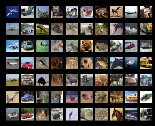
显示样本

# Visualize some examples from the dataset.
# We show a few examples of training images from each class.
classes = ['plane', 'car', 'bird', 'cat', 'deer', 'dog', 'frog', 'horse', 'ship', 'truck']
num_classes = len(classes)
samples_per_class = 7
for y, cls in enumerate(classes):
    idxs = np.flatnonzero(y_train == y)
    idxs = np.random.choice(idxs, samples_per_class, replace=False)
    for i, idx in enumerate(idxs):
        plt_idx = i * num_classes + y + 1
        plt.subplot(samples_per_class, num_classes, plt_idx)
        plt.imshow(X_train[idx].astype('uint8'))
        plt.axis('off')
        if i == 0:
            plt.title(cls)
plt.show()

OUTPUT:

numpy.flatnonzero():
该函数输入一个矩阵，返回扁平化后矩阵中非零元素的位置（index）

enumerate()
返回一个可迭代对象的枚举形式，（上面第一个 返回 0 plane/ 1 car/ 2 bird/……）

调整数据集大小

# Subsample the data for more efficient code execution in this exercise
num_training = 5000
mask = range(num_training)
X_train = X_train[mask]
y_train = y_train[mask]

num_test = 500
mask = range(num_test)
X_test = X_test[mask]
y_test = y_test[mask]

# 把一张图片变为一行向量
X_train = np.reshape(X_train, (X_train.shape[0], -1))
X_test = np.reshape(X_test, (X_test.shape[0], -1))
print(X_train.shape, X_test.shape)

OUTPUT：(5000, 3072) (500, 3072)

KNN模型实现

在cs231n\classifiers文件夹中的 k_nearest_neighbor.py 完成KNN的实现代码。
由于每一个图片用一行数据来表示，要得到测试图片 j 与训练图片 i 的L2距离：

只需要将测试数据矩阵第 j 行的每一个点与训练数据矩阵 第 i 行的每一个点平方求和再开方：

dist[i,j]=np.sqrt(np.sum(np.square(self.X_train[j,:]-X_test[i,:])))

具体如下：

import numpy as np
from collections import Counter

class KNearestNeighbor(object):
  """ a kNN classifier with L2 distance """

  def __init__(self):
    pass

  def train(self, X, y):

    self.X_train = X
    self.y_train = y

  def predict(self, X, k=1, num_loops=0):

    if num_loops == 0:
      dists = self.compute_distances_no_loops(X)
    elif num_loops == 1:
      dists = self.compute_distances_one_loop(X)
    elif num_loops == 2:
      dists = self.compute_distances_two_loops(X)
    else:
      raise ValueError('Invalid value %d for num_loops' % num_loops)

    return self.predict_labels(dists, k=k)

  def compute_distances_two_loops(self, X):

    num_test = X.shape[0]
    num_train = self.X_train.shape[0]
    dists = np.zeros((num_test, num_train))
    for i in range(num_test):#测试样本的循环
      for j in range(num_train):#训练样本的循环            
        #dists[i,j]=np.sqrt(np.sum(np.square(self.X_train[j,:]-X[i,:])))
        dists[i,j]=np.linalg.norm(X[i]-self.X_train[j])
        #np.square是针对每个元素的平方方法  
    return dists

  def compute_distances_one_loop(self, X):

    num_test = X.shape[0]
    num_train = self.X_train.shape[0]
    dists = np.zeros((num_test, num_train))
    for i in range(num_test):
      #dists[i,:] = np.sqrt(np.sum(np.square(self.X_train-X[i,:]),axis = 1))
      dists[i,:]=np.linalg.norm(X[i,:]-self.X_train[:],axis=1)
    return dists

  def compute_distances_no_loops(self, X):
    num_test = X.shape[0]
    num_train = self.X_train.shape[0]
    dists = np.zeros((num_test, num_train)) 
    """
    mul1 = np.multiply(np.dot(X,self.X_train.T),-2)   
    sq1 = np.sum(np.square(X),axis=1,keepdims = True)   
    sq2 = np.sum(np.square(self.X_train),axis=1)   
    dists = mul1+sq1+sq2    
    dists = np.sqrt(dists) 
    """
    dists += np.sum(np.multiply(X,X),axis=1,keepdims = True).reshape(num_test,1)
    dists += np.sum(np.multiply(self.X_train,self.X_train),axis=1,keepdims = True).reshape(1,num_train)
    dists += -2*np.dot(X,self.X_train.T)
    dists = np.sqrt(dists) 

    return dists

  def predict_labels(self, dists, k=1):

    num_test = dists.shape[0]
    y_pred = np.zeros(num_test)
    for i in range(num_test):

        closest_y = []
        closest_y = self.y_train[np.argsort(dists[i, :])[:k]].flatten()
        c = Counter(closest_y)
        y_pred[i]=c.most_common(1)[0][0]
        """
        closest_y=self.y_train[np.argsort(dists[i, :])[:k]]      
        y_pred[i] = np.argmax(np.bincount(closest_y))
        """

    return y_pred

numpy.bincount详见这里

训练模型

knn.ipynb：导入KNN模型

from cs231n.classifiers import KNearestNeighbor

classifier = KNearestNeighbor()
classifier.train(X_train, y_train)

dists = classifier.compute_distances_two_loops(X_test)
print (dists.shape) #>> (500,5000)

y_test_pred = classifier.predict_labels(dists, k=1)

#计算两层循环的结果
num_correct = np.sum(y_test_pred == y_test)
accuracy = float(num_correct) / num_test
print ('Got %d / %d correct => accuracy: %f' % (num_correct, num_test, accuracy))
#>>Got 137 / 500 correct => accuracy: 0.274000
#计算一层循环的结果
y_test_pred = classifier.predict_labels(dists, k=5)
num_correct = np.sum(y_test_pred == y_test)
accuracy = float(num_correct) / num_test
print ('Got %d / %d correct => accuracy: %f' % (num_correct, num_test, accuracy))
#>>Got 139 / 500 correct => accuracy: 0.278000

dists_one = classifier.compute_distances_one_loop(X_test)
#检查两次距离是否一样 dists，dists_one
difference = np.linalg.norm(dists - dists_one, ord='fro')
print ('Difference was: %f' % (difference, ))
if difference < 0.001:
  print ('Good! The distance matrices are the same')
else:
  print ('Uh-oh! The distance matrices are different')

dists_two = classifier.compute_distances_no_loops(X_test)

#检查两次距离是否一样 dists，dists_two
difference = np.linalg.norm(dists - dists_two, ord='fro')
print ('Difference was: %f' % (difference, ))
if difference < 0.001:
  print ('Good! The distance matrices are the same')
else:
  print ('Uh-oh! The distance matrices are different')

计算花费的时间

# Let's compare how fast the implementations are
def time_function(f, *args):
  """
  Call a function f with args and return the time (in seconds) that it took to execute.
  """
  import time
  tic = time.time()
  f(*args)
  toc = time.time()
  return toc - tic

two_loop_time = time_function(classifier.compute_distances_two_loops, X_test)
print ('Two loop version took %f seconds' % two_loop_time)

one_loop_time = time_function(classifier.compute_distances_one_loop, X_test)
print ('One loop version took %f seconds' % one_loop_time)

no_loop_time = time_function(classifier.compute_distances_no_loops, X_test)
print ('No loop version took %f seconds' % no_loop_time)

OUTPUT：
Two loop version took 54.055462 seconds
One loop version took 125.000361 seconds
No loop version took 0.686570 seconds

利用Cross-validation选择K值

超参数 hyperparameter
机器学习算法设计中，如K-NN中的k的取值，以及计算像素差异时使用的距离公式，都是超参数，而调参更是机器学习中不可或缺的一步。
注意：调参要用validation set,而不是test set. 机器学习算法中，测试集只能被用作最后测试，得出结论，如果之前用了，就会出现过拟合的情况

交叉验证cross validation set
这是当训练集数量较小的时候，可以将训练集平分成几份，然后循环取出一份当做validation set 然后把每次结果最后取平均。如下：
将训练集分为如下几部分：

num_folds = 5
k_choices = [1, 3, 5, 8, 10, 12, 15, 20, 50, 100]

X_train_folds = []
y_train_folds = []

X_train_folds = np.array_split(X_train, num_folds)
y_train_folds = np.array_split(y_train, num_folds)

k_to_accuracies = {}

for k in k_choices:
    k_to_accuracies[k] = np.zeros(num_folds)
    for i in range(num_folds):
        Xtr = np.array(X_train_folds[:i] + X_train_folds[i+1:])
        ytr = np.array(y_train_folds[:i] + y_train_folds[i+1:])
        Xte = np.array(X_train_folds[i])
        yte = np.array(y_train_folds[i])     

        Xtr = np.reshape(Xtr, (X_train.shape[0] * 4 / 5, -1))
        ytr = np.reshape(ytr, (y_train.shape[0] * 4 / 5, -1))
        Xte = np.reshape(Xte, (X_train.shape[0] / 5, -1))
        yte = np.reshape(yte, (y_train.shape[0] / 5, -1))

        classifier.train(Xtr, ytr)
        yte_pred = classifier.predict(Xte, k)
        yte_pred = np.reshape(yte_pred, (yte_pred.shape[0], -1))
        num_correct = np.sum(yte_pred == yte)
        accuracy = float(num_correct) / len(yte)
        k_to_accuracies[k][i] = accuracy
# Print out the computed accuracies
for k in sorted(k_to_accuracies):
    for accuracy in k_to_accuracies[k]:
        print ('k = %d, accuracy = %f' % (k, accuracy))

OUTPUT:
k = 1, accuracy = 0.263000
k = 1, accuracy = 0.257000
k = 1, accuracy = 0.264000
k = 1, accuracy = 0.278000
k = 1, accuracy = 0.266000
k = 3, accuracy = 0.241000
k = 3, accuracy = 0.249000
k = 3, accuracy = 0.243000
k = 3, accuracy = 0.273000
k = 3, accuracy = 0.264000
k = 5, accuracy = 0.258000
k = 5, accuracy = 0.273000
k = 5, accuracy = 0.281000
k = 5, accuracy = 0.290000
k = 5, accuracy = 0.272000
k = 8, accuracy = 0.263000
k = 8, accuracy = 0.288000
k = 8, accuracy = 0.278000
k = 8, accuracy = 0.285000
k = 8, accuracy = 0.277000
k = 10, accuracy = 0.265000
k = 10, accuracy = 0.296000
k = 10, accuracy = 0.278000
k = 10, accuracy = 0.284000
k = 10, accuracy = 0.286000
k = 12, accuracy = 0.260000
k = 12, accuracy = 0.294000
k = 12, accuracy = 0.281000
k = 12, accuracy = 0.282000
k = 12, accuracy = 0.281000
k = 15, accuracy = 0.255000
k = 15, accuracy = 0.290000
k = 15, accuracy = 0.281000
k = 15, accuracy = 0.281000
k = 15, accuracy = 0.276000
k = 20, accuracy = 0.270000
k = 20, accuracy = 0.281000
k = 20, accuracy = 0.280000
k = 20, accuracy = 0.282000
k = 20, accuracy = 0.284000
k = 50, accuracy = 0.271000
k = 50, accuracy = 0.288000
k = 50, accuracy = 0.278000
k = 50, accuracy = 0.269000
k = 50, accuracy = 0.266000
k = 100, accuracy = 0.256000
k = 100, accuracy = 0.270000
k = 100, accuracy = 0.263000
k = 100, accuracy = 0.256000
k = 100, accuracy = 0.263000

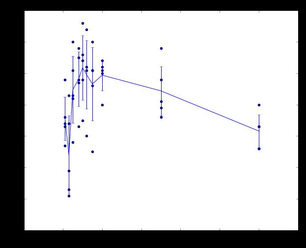
# plot the raw observations
for k in k_choices:
  accuracies = k_to_accuracies[k]
  plt.scatter([k] * len(accuracies), accuracies)

# plot the trend line with error bars that correspond to standard deviation
accuracies_mean = np.array([np.mean(v) for k,v in sorted(k_to_accuracies.items())])
accuracies_std = np.array([np.std(v) for k,v in sorted(k_to_accuracies.items())])
plt.errorbar(k_choices, accuracies_mean, yerr=accuracies_std)
plt.title('Cross-validation on k')
plt.xlabel('k')
plt.ylabel('Cross-validation accuracy')
plt.show()

OUTPUT:

基于交叉验证集选出合适的K值

# Based on the cross-validation results above, choose the best value for k,   
# retrain the classifier using all the training data, and test it on the test
# data. You should be able to get above 28% accuracy on the test data.
best_k = 5
classifier = KNearestNeighbor()
classifier.train(X_train, y_train)
y_test_pred = classifier.predict(X_test, k=best_k)

# Compute and display the accuracy
num_correct = np.sum(y_test_pred == y_test)
accuracy = float(num_correct) / num_test
print ('Got %d / %d correct => accuracy: %f' % (num_correct, num_test, accuracy))
#>>Got 142 / 500 correct => accuracy: 0.284000