GluonTS - Probabilistic Time Series Modeling

GluonTS is a toolkit for building time series models based on deep learning and probabilistic modeling techniques.

1. Installation

1. Create and activate virtual enviroment for mxnet

sudo apt install python3-venv
python3 -m venv my-project-env
source my-project-env/bin/activate

2. GluonTS requires Python 3.6

$ python
Python 3.6.9 (default, Nov  7 2019, 10:44:02) 
[GCC 8.3.0] on linux

4. Update pip and install gluonts

$ pip3 install --upgrade pip
$ pip install --upgrade mxnet==1.4.1 gluonts

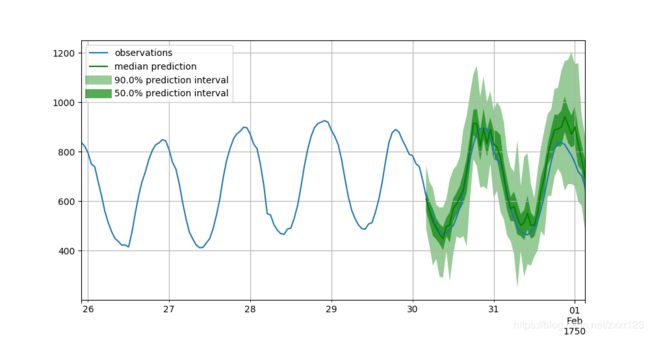
5. Run the quick example code

import pandas as pd
url = "https://raw.githubusercontent.com/numenta/NAB/master/data/realTweets/Twitter_volume_AMZN.csv"
df = pd.read_csv(url, header=0, index_col=0)

import matplotlib.pyplot as plt
df[:100].plot(linewidth=2)
plt.grid(which='both')
plt.show()

from gluonts.dataset.common import ListDataset
training_data = ListDataset(
    [{"start": df.index[0], "target": df.value[:"2015-04-05 00:00:00"]}],
    freq = "5min"
)

from gluonts.model.deepar import DeepAREstimator
from gluonts.trainer import Trainer

estimator = DeepAREstimator(freq="5min", prediction_length=12, trainer=Trainer(epochs=10))
predictor = estimator.train(training_data=training_data)

test_data = ListDataset(
    [{"start": df.index[0], "target": df.value[:"2015-04-15 00:00:00"]}],
    freq = "5min"
)

from gluonts.dataset.util import to_pandas

for test_entry, forecast in zip(test_data, predictor.predict(test_data)):
    to_pandas(test_entry)[-100:].plot(linewidth=2)
    forecast.plot(color='g', prediction_intervals=[50.0, 90.0])
plt.grid(which='both')
plt.legend(["past observations", "median prediction", "90% prediction interval", "50% prediction interval"])
plt.show()

2. Introduction

GluonTS is a toolkit for building time series models based on deep learning and probabilistic modeling techniques. It is not intended as a forecasting solution for businesses or end users but it rather targets scientists and engineers who want to tweak algorithms or build and experiment with their own models.

GluonTS包含了一些已经发布的深度学习模型. 由于深度学习模型的训练难以解释且需要很强算力，因此集成基于公开数据训练的模型是个好主意。在实际应用中可能需要对训练这些模型的基础数据及模型结构有所了解，才能与自己的实际问题充分结合。(To show-case its model building capabilities and facilitate benchmarking, it comes with implementations for a number of already published models).

A Box-Cox transformation is a way to transform non-normal dependent variables into a normal shape

2.1 Time Series Problems

时间序列问题，以单变量（uni-variate）或多变量（multi-variate）时间序列数据为基础重点是3方面应用
（1）预测forecast
（2）平滑插值smooth。本质上是一种预测，只不过这种预测不是针对未来，而是针对缺失或没观测到的值。这类问题的目标是估计这些缺省值的（联合）概率分布。除了一般的方法外，可以应用sequence structure来使用一些比较复杂的方式。(Smoothing or missing value imputation in time series can leverage the sequence structure, and therefore allow for more sophisticated approaches compared to the general missing value imputation setting. Missing values are commonly found in real-world time series collections. For instance, in retail demand forecasting, the true demand is not observed when the item is not in-stock, i.e., cannot be sold. Smoothing is similar to forecasting, except that the time points that we want to predict do not lie in the future. Instead, for a set of series and arbitrary time points there are missing or unobserved values, and the goal is to estimate the (joint) probability distribution over these missing values )
（3）异常探测anomaly detection。实际应用环境中，由于anomaly或outlier是很稀少的；因此这类问题，通常是在处于非监督类情况下的，类似预测问题。这类预测的问题的特征是已经知道或观测到具体的值，但需要知道出现这个值的可能性（即概率）。

• 对于单变量模型，核心是cumulative distribution function.
• 对于多变量模型，核心是the log-likelihood values. 这个值取决于模型及训练数据。
  这两种方式，既可以标记异常点，也可以标记异常序列。异常探测模型质量取决于训练数据中的异常值的出现频率，若能人为删除异常值则有助于异常探测模型的质量。同时，这些training data中的这些异常值，可用于设置可能性的阈值或评估模型准确性。
  (In this unsupervised case, anomaly detection is similar to forecasting, except that all values are observed and we want to know how likely they were. A probabilistic forecasting model can be converted into an anomaly detection model in different ways.
  For univariate models where the cumulative distribution function (CDF) of the marginal predicted distribution can be evaluated, one can directly calculate the p-value (tail probability) of a newly observed data point via the CDF.
  For other models or in the multivariate case, we can use the log-likelihood values. This is slightly more complicated, since the range of log-likelihood values depends on the model and the dataset, however, we can estimate multiple high percentiles of the distribution of negative log-likelihood values on the training set, such as the 99, 99.9, 99.99 etc. At prediction time, we can evaluate the negative log-likelihood of each observations under the model sequentially, and compare this with the estimated quantiles.
  Both approaches allow us to mark unlikely points or unlikely sequences of observations as anomalies. The quality of this forecasting based approach depends on the frequency of such anomalies in the training data, and works best if known anomalies are removed or masked. If some labels for anomalous points are available, they can be used to set likelihood thresholds or to evaluate model accuracy e.g. by calculating classification scores, such as precision and recall.)

2.2 Time Series Models

经典模型的参数取决于每个具体的时间序列。近期，通过共享模型参数，训练生成适用所有时间序列的单一神经网络模型。

通过实验，对不同的数据集，GluonTS软件包中的7种模型表现不一。

• Auto-ARIMA
• Auto-ETS
• Prophet
• NPTS(Non-Parametric Time Series)
• Transformer
• CNN-QR
• Deep-AR

3. Quick Start Tutorial

3.1 Custom datasets

自定义的数据，要想适用GluonTS，需要经过2步：

1. 时间序列的index用pandas.Timestamp来定义，具体数值为numpy.array类型.
2. 利用ListDataset生成GluonTS识别的数据格式，这一数据格式中至少需包含start和target两个关键词。start指代时间序列的index，target指代具体时间序列数值。（In general, a dataset should satisfy some minimum format requirements to be compatible with GluonTS. In particular, it should be an iterable collection of data entries (time series), and each entry should have at least a target field, which contains the actual values of the time series, and astart field, which denotes the starting date of the time series. ）
   这样能确保数据iterable，这是指数据能够一次加载且在for循环中逐个访问。

The only requirements for a custom dataset are to be iterable and have a “target” and a “start” field. To make this more clear, assume the common case where a dataset is in the form of a numpy.array and the index of the time series in a pandas.Timestamp (possibly different for each time series):

N = 10  # number of time series
T = 100  # number of timesteps
prediction_length = 24
freq = "1H"
custom_dataset = np.random.normal(size=(N, T))
start = pd.Timestamp("01-01-2019", freq=freq)  # can be different for each time series

# Now, you can split your dataset and bring it in a GluonTS appropriate format with just two lines of code:

from gluonts.dataset.common import ListDataset


# train dataset: cut the last window of length "prediction_length", add "target" and "start" fields
train_ds = ListDataset([{'target': x, 'start': start} 
                        for x in custom_dataset[:, :-prediction_length]],
                       freq=freq)
# test dataset: use the whole dataset, add "target" and "start" fields
test_ds = ListDataset([{'target': x, 'start': start} 
                       for x in custom_dataset],
                      freq=freq)

3.2 Training an existing model

GluonTS中包含一些预置模型，这些模型的具体命令都以Estimator为结尾。在自定义数据的基础上，人为定义一些特定模型的超参数(hyperparameters such as prediction_length, num_hidden_dimensions specific for neural network, the stride in CNN)之后，就是要通过训练，估算（Estimate）这些预置模型的一些系数、权重等（coefficients, weights, etc）。

from gluonts.model.simple_feedforward import SimpleFeedForwardEstimator
from gluonts.trainer import Trainer


estimator = SimpleFeedForwardEstimator(
    num_hidden_dimensions=[10],
    prediction_length=dataset.metadata.prediction_length,
    context_length=100,
    freq=dataset.metadata.freq,
    trainer=Trainer(ctx="cpu", 
                    epochs=5, 
                    learning_rate=1e-3, 
                    num_batches_per_epoch=100
                   )
)

# After specifying our estimator with all the necessary hyperparameters we can train it using our training dataset `dataset.train` by invoking the `train` method of the estimator. The training algorithm returns a fitted model (or a `Predictor` in GluonTS parlance) that can be used to construct forecasts.

predictor = estimator.train(dataset.train)

训练使用的是GluonTS自带的数据集。训练完后，就可以用predictor来预测。GluonTS中的make_evaluation_predictions可以自动做预测和模型评估；首先删掉test数据中尾部的预测窗口内数据，这也表明test数据中必须包含实际的测试数据；其次，利用剩下的数据做预测，当然预测就是删除的；最后，输出预测结果。

from gluonts.evaluation.backtest import make_evaluation_predictions

forecast_it, ts_it = make_evaluation_predictions(
    dataset=dataset.test,  # test dataset
    predictor=predictor,  # predictor
    num_samples=100,  # number of sample paths we want for evaluation
)

forecasts = list(forecast_it)
tss = list(ts_it)

ts_entry = tss[0]
forecast_entry = forecasts[0]


def plot_prob_forecasts(ts_entry, forecast_entry):
    plot_length = 150 
    prediction_intervals = (50.0, 90.0)
    legend = ["observations", "median prediction"] + [f"{k}% prediction interval" for k in prediction_intervals][::-1]

    fig, ax = plt.subplots(1, 1, figsize=(10, 7))
    ts_entry[-plot_length:].plot(ax=ax)  # plot the time series
    forecast_entry.plot(prediction_intervals=prediction_intervals, color='g')
    plt.grid(which="both")
    plt.legend(legend, loc="upper left")
    plt.show()

plot_prob_forecasts(ts_entry, forecast_entry)

定量评估模型精度：

>>> from gluonts.evaluation import Evaluator
>>> evaluator = Evaluator(quantiles=[0.1, 0.5, 0.9])
>>> 
>>> agg_metrics, item_metrics = evaluator(iter(tss), iter(forecasts), num_series=len(dataset.test))
Running evaluation: 100%|█████████████████████████████████████████| 414/414 [00:01<00:00, 270.12it/s]
>>> # Aggregate metrics aggregate both across time-steps and across time series.
>>> print(json.dumps(agg_metrics, indent=4))
{
    "MSE": 11472922.553122135,
    "abs_error": 10421132.363254547,
    "abs_target_sum": 145558863.59960938,
    "abs_target_mean": 7324.822041043146,
    "seasonal_error": 336.9046924038305,
    "MASE": 3.3453605150604617,
    "sMAPE": 0.18586365287131185,
    "MSIS": 36.96800237470267,
    "QuantileLoss[0.1]": 4783764.862509155,
    "Coverage[0.1]": 0.09636674718196456,
    "QuantileLoss[0.5]": 10421132.352004051,
    "Coverage[0.5]": 0.5744766505636071,
    "QuantileLoss[0.9]": 7613085.972868537,
    "Coverage[0.9]": 0.8880837359098229,
    "RMSE": 3387.170286998003,
    "NRMSE": 0.4624235603293412,
    "ND": 0.07159393873752744,
    "wQuantileLoss[0.1]": 0.03286481320483456,
    "wQuantileLoss[0.5]": 0.07159393866023572,
    "wQuantileLoss[0.9]": 0.0523024554094483,
    "mean_wQuantileLoss": 0.05225373575817286,
    "MAE_Coverage": 0.030008722490606543
}

item_metrics.plot(x='MSIS', y='MASE', kind='scatter')
plt.grid(which="both")
plt.show()

要想研究明白这些衡量准确性的指标，还需要仔细学习一下，目前找到2篇论文：

1. The M3-Competition: results, conclusions and implications
2. Another look at measures of forecast accuracy.The data of this paper
   MASE: Mean Absolute Scaled Error proposed by Koehler & Hyndman (2006).

$$MASE=\frac{MAE}{MA{E}_{in-sample,navie}}=\frac{1}{h}\frac{{\sum }_{t=1}^h|Y_t-\widehat{Y_t}|}{\frac{1}{n-m}{\sum }_{t=m+1}^n|Y_t-Y_{t-m}|}$$

where MAE is the mean absolute error produced by the actual forecast;
while $MA{E}_{in-sample,naive}$ is the mean absolute error produced by a naive forecast (e.g. no-change forecast for an integrated $I(1)$ time series), calculated on the in-sample data.
$MASE>1$ implies that the actual forecast does worse out of sample than a naive forecast did in sample, in terms of mean absolute error.Source

sMAPE: the symmetric Mean Absolute Percentage Error
$$sMAPE=\frac{1}{h}\sum _{t=1}^h\frac{2|Y_t-\widehat{Y_t}|}{|Y_t|+|\widehat{Y_t}|}$$

• $Y_t$ is the post sample value of the time series at point $t$.
• $\widehat{Y_t}$ is the estimated forecast.
• $h$ is the forecasting horizon.
• $m$ is the frequency of the data.
  Competitor’s Guide: Prizes and Rules

迄今为止发现的最好用的markdown中输入数学公式的资料LATEX Mathematical Symbols，为了输入$\hat{Y}$，找了半天。

3.3 Create your own forecast model

创建预测模型要做2部分：

1. 定义训练网络和预测网络
2. Define a new estimator that specifies any data processing and uses the networks

3.3.1 Define the training and prediction network

自定义的训练网络和预测网络，也是2个class，需要都包含hybrid_forward。训练网络中的hybrid_forward应该返回预测值和观测值之间的loss，预测网络中的hybrid_forward应该返回预测值。为确保预测网络与训练网络的一致性，预测网络是直接继承（inherit）训练网络。

class MyTrainNetwork(gluon.HybridBlock):
    def __init__(self, prediction_length, **kwargs):
        super().__init__(**kwargs)
        self.prediction_length = prediction_length

        with self.name_scope():
            # Set up a 3 layer neural network that directly predicts the target values
            self.nn = mx.gluon.nn.HybridSequential()
            self.nn.add(mx.gluon.nn.Dense(units=40, activation='relu'))
            self.nn.add(mx.gluon.nn.Dense(units=40, activation='relu'))
            self.nn.add(mx.gluon.nn.Dense(units=self.prediction_length, activation='softrelu'))

    def hybrid_forward(self, F, past_target, future_target):
        prediction = self.nn(past_target)
        # calculate L1 loss with the future_target to learn the median
        return (prediction - future_target).abs().mean(axis=-1)

class MyPredNetwork(MyTrainNetwork):
    # The prediction network only receives past_target and returns predictions
    def hybrid_forward(self, F, past_target):
        prediction = self.nn(past_target)
        return prediction.expand_dims(axis=1)

3.3.2 Define a new estimator

定义estimator需要包含以下3个方法：

1. create_transformation定义所有feature transformation和训练期间数据如何切分。
2. create_training_network通过配置必要的hyperparameters返回训练网络。
3. create_predictor实现预测网络并返回Predictor对象。

from gluonts.model.estimator import GluonEstimator
from gluonts.model.predictor import Predictor, RepresentableBlockPredictor
from gluonts.core.component import validated
from gluonts.support.util import copy_parameters
from gluonts.transform import ExpectedNumInstanceSampler, Transformation, InstanceSplitter
from gluonts.dataset.field_names import FieldName
from mxnet.gluon import HybridBlock

class MyEstimator(GluonEstimator):
    @validated()
    def __init__(
        self,
        freq: str,
        context_length: int,
        prediction_length: int,
        trainer: Trainer = Trainer()
    ) -> None:
        super().__init__(trainer=trainer)
        self.context_length = context_length
        self.prediction_length = prediction_length
        self.freq = freq


    def create_transformation(self):
        # Feature transformation that the model uses for input.
        # Here we use a transformation that randomly select training samples from all time series.
        return InstanceSplitter(
                    target_field=FieldName.TARGET,
                    is_pad_field=FieldName.IS_PAD,
                    start_field=FieldName.START,
                    forecast_start_field=FieldName.FORECAST_START,
                    train_sampler=ExpectedNumInstanceSampler(num_instances=1),
                    past_length=self.context_length,
                    future_length=self.prediction_length,
                )

    def create_training_network(self) -> MyTrainNetwork:
        return MyTrainNetwork(
            prediction_length=self.prediction_length
        )

    def create_predictor(
        self, transformation: Transformation, trained_network: HybridBlock
    ) -> Predictor:
        prediction_network = MyPredNetwork(
            prediction_length=self.prediction_length
        )

        copy_parameters(trained_network, prediction_network)

        return RepresentableBlockPredictor(
            input_transform=transformation,
            prediction_net=prediction_network,
            batch_size=self.trainer.batch_size,
            freq=self.freq,
            prediction_length=self.prediction_length,
            ctx=self.trainer.ctx,
        )

下面就是训练网络、开展预测。

estimator = MyEstimator(
    prediction_length=dataset.metadata.prediction_length,
    context_length=100,
    freq=dataset.metadata.freq,
    trainer=Trainer(ctx="cpu", 
                    epochs=5, 
                    learning_rate=1e-3, 
                    num_batches_per_epoch=100
                   )
)

predictor = estimator.train(dataset.train)

forecast_it, ts_it = make_evaluation_predictions(
    dataset=dataset.test,
    predictor=predictor,
    num_samples=100
)

forecasts = list(forecast_it)
tss = list(ts_it)

plot_prob_forecasts(tss[0], forecasts[0])

由于定义的神经网络模型中未做概率预测，因此上图中仅有point estimates。

下面是评估计算结果

>>> evaluator = Evaluator(quantiles=[0.1, 0.5, 0.9])
>>> agg_metrics, item_metrics = evaluator(iter(tss), iter(forecasts), num_series=len(dataset.test))Running evaluation: 100%|███████████████████████████████████████| 414/414 [00:01<00:00, 287.43it/s]
>>> print(json.dumps(agg_metrics, indent=4))
{
    "MSE": 10607463.826149326,
    "abs_error": 10632605.368728638,
    "abs_target_sum": 145558863.59960938,
    "abs_target_mean": 7324.822041043146,
    "seasonal_error": 336.9046924038305,
    "MASE": 4.563430532890973,
    "sMAPE": 0.22919137849889548,
    "MSIS": 182.5372197601393,
    "QuantileLoss[0.1]": 11152860.887708187,
    "Coverage[0.1]": 0.4288949275362319,
    "QuantileLoss[0.5]": 10632605.347156048,
    "Coverage[0.5]": 0.4288949275362319,
    "QuantileLoss[0.9]": 10112349.806603909,
    "Coverage[0.9]": 0.4288949275362319,
    "RMSE": 3256.9101655018558,
    "NRMSE": 0.4446401765466006,
    "ND": 0.07304677369545753,
    "wQuantileLoss[0.1]": 0.07662096702256829,
    "wQuantileLoss[0.5]": 0.07304677354725227,
    "wQuantileLoss[0.9]": 0.06947258007193624,
    "mean_wQuantileLoss": 0.07304677354725227,
    "MAE_Coverage": 0.2903683574879227
}
>>> item_metrics.head(10)
   item_id           MSE      abs_error  ...  Coverage[0.5]  QuantileLoss[0.9]  Coverage[0.9]
0      NaN  3.952474e+03    2359.563721  ...       0.333333        2621.275647       0.333333
1      NaN  1.335598e+05   14243.525391  ...       0.854167        4122.227075       0.854167
2      NaN  5.972961e+04    9963.423828  ...       0.145833       16990.749988       0.145833
3      NaN  3.200988e+05   22316.441406  ...       0.291667       28871.196875       0.291667
4      NaN  1.213484e+05   12010.902344  ...       0.437500       15203.732861       0.437500
5      NaN  2.572568e+05   19220.041016  ...       0.583333       18093.033301       0.583333
6      NaN  1.483986e+07  140121.781250  ...       0.291667      225668.073047       0.291667
7      NaN  9.729216e+06  122671.953125  ...       0.333333      171962.992969       0.333333
8      NaN  1.273295e+07  129166.195312  ...       0.687500       62510.790234       0.687500
9      NaN  8.011777e+02    1049.667969  ...       0.187500        1641.506708       0.187500

[10 rows x 15 columns]
>>> item_metrics.plot(x='MSIS', y='MASE', kind='scatter')
<matplotlib.axes._subplots.AxesSubplot object at 0x7f5a01726748>
>>> plt.grid(which="both")
>>> plt.show()

4. Extended Forecasting Tutorial

4.1 Datasets

4.1.1 The datasets provided by GluonTS

4.1.2 Create artificial datasets

4.1.3 Use your time series and features

>>> from gluonts.dataset.field_names import FieldName
>>> [f"FieldName.{k} = '{v}'" for k, v in FieldName.__dict__.items() if not k.startswith('_')]
["FieldName.ITEM_ID = 'item_id'", 
"FieldName.START = 'start'", 
"FieldName.TARGET = 'target'", 
"FieldName.FEAT_STATIC_CAT = 'feat_static_cat'", 
"FieldName.FEAT_STATIC_REAL = 'feat_static_real'", 
"FieldName.FEAT_DYNAMIC_CAT = 'feat_dynamic_cat'", 
"FieldName.FEAT_DYNAMIC_REAL = 'feat_dynamic_real'", 
"FieldName.FEAT_TIME = 'time_feat'", 
"FieldName.FEAT_CONST = 'feat_dynamic_const'", 
"FieldName.FEAT_AGE = 'feat_dynamic_age'", 
"FieldName.OBSERVED_VALUES = 'observed_values'", 
"FieldName.IS_PAD = 'is_pad'", 
"FieldName.FORECAST_START = 'forecast_start'"]

这些字段分为3类：

• 必需的(Required)
• 可选的(Optional)
• 通过Transformation添加的(Added by Transformation)

Required:

• start: start date of the time series
• target: values of the time series

Optional:
feat 是 features首4个字母，这样看名字就知道这个字段的意思了。

• feat_static_cat: static (over time) categorical features, list with dimension equal to the number of features
• feat_static_real: static (over time) real features, list with dimension equal to the number of features
• feat_dynamic_cat: dynamic (over time) categorical features, array with shape equal to (number of features, target length)
• feat_dynamic_real: dynamic (over time) real features, array with shape equal to (number of features, target length). Refer to the issue of adding holidays into the model on github, the holidays and weekends indicator should be added to this field.

Added by Transformation:

• time_feat: time related features such as the month or the day
• feat_dynamic_const: expands a constant value feature along the time axis
• feat_dynamic_age: age feature, i.e., a feature that its value is small for distant past timestamps and it monotonically(单调地) increases the more we approach the current timestamp
• observed_values: indicator for observed values, i.e., a feature that equals to 1 if the value is observed and 0 if the value is missing
• is_pad: indicator for each time step that shows if it is padded (if the length is not enough)
• forecast_start: forecast start date

4.2 Transformation

4.2.1 Define a transformation

Feature processiong,e.g.,adding a holiday feature and for defining the way the dataset will be split into appropriate windows during training and inference.

The Transformation always needs to define how the datasets are going to be split in example windows during training and testing. This is done with the InstanceSplitter that is configured as follows (skipping the obvious fields):

• is_pad_field: indicator if the time series is padded (if the length is not enough)
• train_sampler: defines how the training windows are cut/sampled
• time_series_fields: contains the time dependent features that need to be split in the same manner as the target

from gluonts.transform import (
    AddAgeFeature,
    AddObservedValuesIndicator,
    Chain,
    ExpectedNumInstanceSampler,
    InstanceSplitter,
    SetFieldIfNotPresent,
)

def create_transformation(freq, context_length, prediction_length):
    return Chain(
        [
            AddObservedValuesIndicator(
                target_field=FieldName.TARGET,
                output_field=FieldName.OBSERVED_VALUES,
            ),
            AddAgeFeature(
                target_field=FieldName.TARGET,
                output_field=FieldName.FEAT_AGE,
                pred_length=prediction_length,
                log_scale=True,
            ),
            InstanceSplitter(
                target_field=FieldName.TARGET,
                is_pad_field=FieldName.IS_PAD,
                start_field=FieldName.START,
                forecast_start_field=FieldName.FORECAST_START,
                train_sampler=ExpectedNumInstanceSampler(num_instances=1),
                past_length=context_length,
                future_length=prediction_length,
                time_series_fields=[
                    FieldName.FEAT_AGE,
                    FieldName.FEAT_DYNAMIC_REAL,
                    FieldName.OBSERVED_VALUES,
                ],
            ),
        ]
    )

4.2.2 Transform a dataset

transformation = create_transformation(custom_ds_metadata['freq'],
                                       2 * custom_ds_metadata['prediction_length'], # can be any appropriate value
                                       custom_ds_metadata['prediction_length'])
train_tf = transformation(iter(train_ds), is_train=True)                    

在转化中，若设置is_train为True，表明生成的train_df中是由若干个片段的时间序列，这些时间序列的起始点和长度是随机的。这时候，以furture_打头的字段长度均等于prediction_length.(The type of train_tf is a generator. When is_train=True in the transformation, the InstanceSplitter iterates over the transformed dataset and cuts windows by selecting randomly a time series and a starting point on that time series (this “randomness” is defined by the train_sampler).)

若设置is_train为False，则InstanceSplitter就切在了时间序列的最末端，以furture_打头的字段长度均等于0.（During inference (is_train=False in the transformation), the splitter always cuts the last window (of length context_length) of the dataset so it can be used to predict the subsequent unknown values of length prediction_length.)

train_tf_entry = next(iter(train_tf))
[k for k in train_tf_entry.keys()]

['start',
 'feat_static_cat',
 'source',
 'past_feat_dynamic_age', # newly added
 'future_feat_dynamic_age', # newly added
 'past_feat_dynamic_real',
 'future_feat_dynamic_real',
 'past_observed_values', # newly added
 'future_observed_values', # newly added
 'past_target', # newly added
 'future_target', # newly added
 'past_is_pad',
 'forecast_start']

通过在依赖时间的字段添加相应的前缀，可以将时间窗口区分为过去与未来。如：past_target指过去的目标值（时间跨度等于context_length），future_target指未来的目标值（时间跨度等于prediction_length）；通过这两者可以计算预测误差。(
It has done one more important thing: it has split the window into past and future and has added the corresponding prefixes to all time dependent fields. This way we can easily use e.g., the past_target field as input and the future_target field to calculate the error of our predictions. Of course, the length of the past is equal to the context_length and of the future equal to the prediction_length.)

上述的手动操作可以用DataLoader来代替，此方法以原始数据和需要转换的字段为输入。

4.3 Training an existing model

在整个的预测时长内，评估每个时间步骤的数据分布；进而从这些数据分布中提取样本，形成sample path。实际应用中，通过提取多个样本并创建多个sample path，以用于数据可视化、模型评估和获取统计指标。(The existing models focus on (but are not limited to) probabilistic forecasting. Probabilistic forecasts are predictions in the form of a probability distribution, rather than simply a single point estimate. Having estimated the future distribution of each time step in the forecasting horizon, we can draw a sample from the distribution at each time step and thus create a “sample path” that can be seen as a possible realization of the future. In practice we draw multiple samples and create multiple sample paths which can be used for visualization, evaluation of the model, to derive statistics, etc.)

4.3.1 Configuring an estimator

4.3.2 Getting a predictor

4.3.3 Saving/Loading an existing model

# save the trained model in tmp/
from pathlib import Path
predictor.serialize(Path("/tmp/"))

# loads it back
from gluonts.model.predictor import Predictor
predictor_deserialized = Predictor.deserialize(Path("/tmp/"))

5. Evaluation

5.1 Getting the forecasts

计算多个sample paths的统计值：

print(f"Mean of the future window:\n {forecast_entry.mean}")
print(f"0.5-quantile (median) of the future window:\n {forecast_entry.quantile(0.5)}")

Mean of the future window:
 [ 0.90204316  0.51493835  0.59364754  0.33699945 -0.02405789 -0.09633367
  0.01381113  0.20371772  0.06646997  0.33810818  0.7028771   0.64642954
  1.2103612   1.452136    1.7268275   1.915122    1.8562789   1.8347268
  2.0133853   1.8212171   1.7021966   1.6202236   1.3553896   1.0855911 ]
0.5-quantile (median) of the future window:
 [ 0.9203323   0.5516612   0.5740295   0.30386427  0.01295065 -0.12111787
  0.06435527  0.16646238  0.01448222  0.34552932  0.72008365  0.67345566
  1.1754254   1.3199731   1.6971017   1.9455458   1.8559864   1.8195658
  2.0560982   1.8159965   1.7261845   1.6376166   1.4088321   1.0873951 ]

5.2 Compute metrics

5.3 Creating your own model

5.3.1 Point forecasts with a simple feedforward network

5.3.2 Probabilistic forecasting

5.3.2.1 How does a model learn a distribution?

要想知道未来每个时间步长的概率分布，先要人为确定一个分布形式（如Gaussian, Student-t and Uniform等）。确定具体的概率分布，是通过学习，每种分布形式的相关参数得到的。GluonTS中每种分布形式对应一个类，这些类定义了每种分布形式的相关参数、(log-)likelihood和取样方法。

Probabilistic forecasting requires that we learn the distribution of the future values of the time series and not the values themselves as in point forecasting. To achieve this, we need to specify the type of distribution that the future values follow. GluonTS comes with a number of different distributions that cover many use cases, such as Gaussian, Student-t and Uniform just to name a few.

In order to learn a distribution we need to learn its parameters. For example, in the simple case where we assume a Gaussian distribution, we need to learn the mean and the variance that fully specify the distribution.

Each distribution that is available in GluonTS is defined by the corresponding Distribution class (e.g., Gaussian). This class defines -among others- the parameters of the distribution, its (log-)likelihood and a sampling method (given the parameters).

在GluonTS中，神经网络模型通过DistributionOutput类（如GaussianOutput类）与某个概率分布相连接。这些类主要将神经网络模型的输出结果映射到分布的具体参数，从而在模型训练过程中得到具体每个时间步长概率分布的参数；训练过程中神经网络模型是通过选定的loss function，概率分布参数的确定是通过选定分布的negative log-likelihood。可以将概率分布层看作神经网络模型顶部附加的projection layer.
However, it is not straightforward how to connect a model with such a distribution and learn its parameters. For this, each distribution comes with a DistributionOutput class (e.g., GaussianOutput). The role of this class is to connect a model with a distribution. Its main usage is to take the output of the model and map it to the parameters of the distribution. You can think of it as an additional projection layer on top of the model. The parameters of this layer are optimized along with the rest of the network.

By including this projection layer, our model effectively learns the parameters of the (chosen) distribution of each time step. Such a model is usually optimized by choosing as a loss function the negative log-likelihood of the chosen distribution. After we optimize our model and learn the parameters we can sample or derive any other useful statistics from the learned distributions.

5.3.2.2 Feedforward network for probabilistic forecasting

from gluonts.distribution.distribution_output import DistributionOutput
from gluonts.distribution.gaussian import GaussianOutput



class MyProbNetwork(gluon.HybridBlock):
    def __init__(self, 
                 prediction_length, 
                 distr_output, 
                 num_cells, 
                 num_sample_paths=100, 
                 **kwargs
    ) -> None:
        super().__init__(**kwargs)
        self.prediction_length = prediction_length
        self.distr_output = distr_output
        self.num_cells = num_cells
        self.num_sample_paths = num_sample_paths
        self.proj_distr_args = distr_output.get_args_proj()

        with self.name_scope():
            # Set up a 2 layer neural network that its ouput will be projected to the distribution parameters
            self.nn = mx.gluon.nn.HybridSequential()
            self.nn.add(mx.gluon.nn.Dense(units=self.num_cells, activation='relu'))
            self.nn.add(mx.gluon.nn.Dense(units=self.prediction_length * self.num_cells, activation='relu'))


class MyProbTrainNetwork(MyProbNetwork):
    def hybrid_forward(self, F, past_target, future_target):
        # compute network output
        net_output = self.nn(past_target)

        # (batch, prediction_length * nn_features)  ->  (batch, prediction_length, nn_features)
        net_output = net_output.reshape(0, self.prediction_length, -1)

        # project network output to distribution parameters domain
        distr_args = self.proj_distr_args(net_output)

        # compute distribution
        distr = self.distr_output.distribution(distr_args)

        # negative log-likelihood
        loss = distr.loss(future_target)
        return loss


class MyProbPredNetwork(MyProbTrainNetwork):
    # The prediction network only receives past_target and returns predictions
    def hybrid_forward(self, F, past_target):
        # repeat past target: from (batch_size, past_target_length) to 
        # (batch_size * num_sample_paths, past_target_length)
        repeated_past_target = past_target.repeat(
            repeats=self.num_sample_paths, axis=0
        )
        
        # compute network output
        net_output = self.nn(repeated_past_target)

        # (batch * num_sample_paths, prediction_length * nn_features)  ->  (batch * num_sample_paths, prediction_length, nn_features)
        net_output = net_output.reshape(0, self.prediction_length, -1)
       
        # project network output to distribution parameters domain
        distr_args = self.proj_distr_args(net_output)

        # compute distribution
        distr = self.distr_output.distribution(distr_args)

        # get (batch_size * num_sample_paths, prediction_length) samples
        samples = distr.sample()
        
        # reshape from (batch_size * num_sample_paths, prediction_length) to 
        # (batch_size, num_sample_paths, prediction_length)
        return samples.reshape(shape=(-1, self.num_sample_paths, self.prediction_length))

#
# The changes we need to do at the estimator are minor and they mainly reflect the additional `distr_output` parameter that our networks use.


class MyProbEstimator(GluonEstimator):
    @validated()
    def __init__(
            self,
            prediction_length: int,
            context_length: int,
            freq: str,
            distr_output: DistributionOutput,
            num_cells: int,
            num_sample_paths: int = 100,
            trainer: Trainer = Trainer()
    ) -> None:
        super().__init__(trainer=trainer)
        self.prediction_length = prediction_length
        self.context_length = context_length
        self.freq = freq
        self.distr_output = distr_output
        self.num_cells = num_cells
        self.num_sample_paths = num_sample_paths

    def create_transformation(self):
        return InstanceSplitter(
            target_field=FieldName.TARGET,
            is_pad_field=FieldName.IS_PAD,
            start_field=FieldName.START,
            forecast_start_field=FieldName.FORECAST_START,
            train_sampler=ExpectedNumInstanceSampler(num_instances=1),
            past_length=self.context_length,
            future_length=self.prediction_length,
        )

    def create_training_network(self) -> MyProbTrainNetwork:
        return MyProbTrainNetwork(
            prediction_length=self.prediction_length,
            distr_output=self.distr_output,
            num_cells=self.num_cells,
            num_sample_paths=self.num_sample_paths
        )

    def create_predictor(
            self, transformation: Transformation, trained_network: HybridBlock
    ) -> Predictor:
        prediction_network = MyProbPredNetwork(
            prediction_length=self.prediction_length,
            distr_output=self.distr_output,
            num_cells=self.num_cells,
            num_sample_paths=self.num_sample_paths
        )

        copy_parameters(trained_network, prediction_network)

        return RepresentableBlockPredictor(
            input_transform=transformation,
            prediction_net=prediction_network,
            batch_size=self.trainer.batch_size,
            freq=self.freq,
            prediction_length=self.prediction_length,
            ctx=self.trainer.ctx,
        )



estimator = MyProbEstimator(
    prediction_length=custom_ds_metadata['prediction_length'],
    context_length=2*custom_ds_metadata['prediction_length'],
    freq=custom_ds_metadata['freq'],
    distr_output=GaussianOutput(),
    num_cells=40,
    trainer=Trainer(ctx="cpu", 
                    epochs=5, 
                    learning_rate=1e-3, 
                    hybridize=False, 
                    num_batches_per_epoch=100
                   )
)



predictor = estimator.train(train_ds)



forecast_it, ts_it = make_evaluation_predictions(
    dataset=test_ds,  # test dataset
    predictor=predictor,  # predictor
    num_samples=100,  # number of sample paths we want for evaluation
)



forecasts = list(forecast_it)
tss = list(ts_it)



plot_prob_forecasts(tss[0], forecasts[0])

5.4 Add features and scaling

添加与目标值一致的feature，与目标值组成一个enhanced vector作为神经王咯模型的输入。
这个例子中仅添加了一个feature，但其实可以添加所有有用的features。
添加了features后，注意一定要做scale. It is extremely helpful for a model to be trained and forecast values that lie roughly in the same value range.

from gluonts.block.scaler import MeanScaler, NOPScaler



class MyProbNetwork(gluon.HybridBlock):
    def __init__(self, 
                 prediction_length, 
                 context_length, 
                 distr_output, 
                 num_cells, 
                 num_sample_paths=100, 
                 scaling=True, 
                 **kwargs
    ) -> None:
        super().__init__(**kwargs)
        self.prediction_length = prediction_length
        self.context_length = context_length
        self.distr_output = distr_output
        self.num_cells = num_cells
        self.num_sample_paths = num_sample_paths
        self.proj_distr_args = distr_output.get_args_proj()
        self.scaling = scaling

        with self.name_scope():
            # Set up a 2 layer neural network that its ouput will be projected to the distribution parameters
            self.nn = mx.gluon.nn.HybridSequential()
            self.nn.add(mx.gluon.nn.Dense(units=self.num_cells, activation='relu'))
            self.nn.add(mx.gluon.nn.Dense(units=self.prediction_length * self.num_cells, activation='relu'))

            if scaling:
                self.scaler = MeanScaler(keepdims=True)
            else:
                self.scaler = NOPScaler(keepdims=True)

    def compute_scale(self, past_target, past_observed_values):
        # scale shape is (batch_size, 1)
        _, scale = self.scaler(
            past_target.slice_axis(
                axis=1, begin=-self.context_length, end=None
            ),
            past_observed_values.slice_axis(
                axis=1, begin=-self.context_length, end=None
            ),
        )

        return scale


class MyProbTrainNetwork(MyProbNetwork):
    def hybrid_forward(self, F, past_target, future_target, past_observed_values, past_feat_dynamic_real):
        # compute scale 
        scale = self.compute_scale(past_target, past_observed_values)

        # scale target and time features
        past_target_scale = F.broadcast_div(past_target, scale)
        past_feat_dynamic_real_scale = F.broadcast_div(past_feat_dynamic_real.squeeze(axis=-1), scale)

        # concatenate target and time features to use them as input to the network
        net_input = F.concat(past_target_scale, past_feat_dynamic_real_scale, dim=-1)

        # compute network output
        net_output = self.nn(net_input)

        # (batch, prediction_length * nn_features)  ->  (batch, prediction_length, nn_features)
        net_output = net_output.reshape(0, self.prediction_length, -1)

        # project network output to distribution parameters domain
        distr_args = self.proj_distr_args(net_output)

        # compute distribution
        distr = self.distr_output.distribution(distr_args, scale=scale)

        # negative log-likelihood
        loss = distr.loss(future_target)
        return loss


class MyProbPredNetwork(MyProbTrainNetwork):
    # The prediction network only receives past_target and returns predictions
    def hybrid_forward(self, F, past_target, past_observed_values, past_feat_dynamic_real):
        # repeat fields: from (batch_size, past_target_length) to
        # (batch_size * num_sample_paths, past_target_length)
        repeated_past_target = past_target.repeat(
            repeats=self.num_sample_paths, axis=0
        )
        repeated_past_observed_values = past_observed_values.repeat(
            repeats=self.num_sample_paths, axis=0
        )
        repeated_past_feat_dynamic_real = past_feat_dynamic_real.repeat(
            repeats=self.num_sample_paths, axis=0
        )
        
        # compute scale
        scale = self.compute_scale(repeated_past_target, repeated_past_observed_values)

        # scale repeated target and time features
        repeated_past_target_scale = F.broadcast_div(repeated_past_target, scale)
        repeated_past_feat_dynamic_real_scale = F.broadcast_div(repeated_past_feat_dynamic_real.squeeze(axis=-1), scale)

        # concatenate target and time features to use them as input to the network
        net_input = F.concat(repeated_past_target_scale, repeated_past_feat_dynamic_real_scale, dim=-1)

        # compute network oputput
        net_output = self.nn(net_input)
        
        # (batch * num_sample_paths, prediction_length * nn_features)  ->  (batch * num_sample_paths, prediction_length, nn_features)
        net_output = net_output.reshape(0, self.prediction_length, -1)

        # project network output to distribution parameters domain
        distr_args = self.proj_distr_args(net_output)
        
        # compute distribution
        distr = self.distr_output.distribution(distr_args, scale=scale)

        # get (batch_size * num_sample_paths, prediction_length) samples
        samples = distr.sample()

        # reshape from (batch_size * num_sample_paths, prediction_length) to
        # (batch_size, num_sample_paths, prediction_length)
        return samples.reshape(shape=(-1, self.num_sample_paths, self.prediction_length))



class MyProbEstimator(GluonEstimator):
    @validated()
    def __init__(
            self,
            prediction_length: int,
            context_length: int,
            freq: str,
            distr_output: DistributionOutput,
            num_cells: int,
            num_sample_paths: int = 100,
            scaling: bool = True,
            trainer: Trainer = Trainer()
    ) -> None:
        super().__init__(trainer=trainer)
        self.prediction_length = prediction_length
        self.context_length = context_length
        self.freq = freq
        self.distr_output = distr_output
        self.num_cells = num_cells
        self.num_sample_paths = num_sample_paths
        self.scaling = scaling

    def create_transformation(self):
        # Feature transformation that the model uses for input.
        return Chain(
            [
                AddObservedValuesIndicator(
                    target_field=FieldName.TARGET,
                    output_field=FieldName.OBSERVED_VALUES,
                ),
                InstanceSplitter(
                    target_field=FieldName.TARGET,
                    is_pad_field=FieldName.IS_PAD,
                    start_field=FieldName.START,
                    forecast_start_field=FieldName.FORECAST_START,
                    train_sampler=ExpectedNumInstanceSampler(num_instances=1),
                    past_length=self.context_length,
                    future_length=self.prediction_length,
                    time_series_fields=[
                        FieldName.FEAT_DYNAMIC_REAL,
                        FieldName.OBSERVED_VALUES,
                    ],
                ),

            ]
        )

    def create_training_network(self) -> MyProbTrainNetwork:
        return MyProbTrainNetwork(
            prediction_length=self.prediction_length,
            context_length=self.context_length,
            distr_output=self.distr_output,
            num_cells=self.num_cells,
            num_sample_paths=self.num_sample_paths,
            scaling=self.scaling
        )

    def create_predictor(
            self, transformation: Transformation, trained_network: HybridBlock
    ) -> Predictor:
        prediction_network = MyProbPredNetwork(
            prediction_length=self.prediction_length,
            context_length=self.context_length,
            distr_output=self.distr_output,
            num_cells=self.num_cells,
            num_sample_paths=self.num_sample_paths,
            scaling=self.scaling
        )

        copy_parameters(trained_network, prediction_network)

        return RepresentableBlockPredictor(
            input_transform=transformation,
            prediction_net=prediction_network,
            batch_size=self.trainer.batch_size,
            freq=self.freq,
            prediction_length=self.prediction_length,
            ctx=self.trainer.ctx,
        )



estimator = MyProbEstimator(
    prediction_length=custom_ds_metadata['prediction_length'],
    context_length=2*custom_ds_metadata['prediction_length'],
    freq=custom_ds_metadata['freq'],
    distr_output=GaussianOutput(),
    num_cells=40,
    trainer=Trainer(ctx="cpu", 
                    epochs=5, 
                    learning_rate=1e-3, 
                    hybridize=False, 
                    num_batches_per_epoch=100
                   )
)



predictor = estimator.train(train_ds)



forecast_it, ts_it = make_evaluation_predictions(
    dataset=test_ds,  # test dataset
    predictor=predictor,  # predictor
    num_samples=100,  # number of sample paths we want for evaluation
)



forecasts = list(forecast_it)
tss = list(ts_it)



plot_prob_forecasts(tss[0], forecasts[0])

5.5 From feedforward to RNN

5.5.1 Training

We can enhance the input by using multiple past values (for example specific lags based on seasonality patterns) or available features.

Due to the sequential nature of the RNN, the distinction between past_ and future_ in the cut window of the time series is not really necessary. Therefore, we can concatenate past_target and future_target and treat it as a concrete target window that we wish to forecast. This means that the input to the RNN would be (sequentially) the window target[-(context_length + prediction_length + 1):-1] (one time step before the window we want to predict). As a consequence, we need to have context_length + prediction_length + 1available values at each window that we cut. We can define this in the InstanceSplitter.

During training the steps are the following:

• We pass sequentially through the RNN the target values target[-(context_length + prediction_length + 1):-1]
• We use the state of the RNN at each time step as a feature vector and project it to the distribution parameter domain
• The output at each time step is the distribution of the values of the next time step, which overall is the forecasted distribution for the window target[-(context_length + prediction_length):]

The above steps are implemented in the unroll_encoder method.

5.5.2 Inference

• We pass sequentially through the RNN the past target values past_target[-(context_length + 1):] that effectively updates the state of the RNN
• In the last time step the output of the RNN is effectively the distribution of the next value of the time series (which we do not know). Therefore we sample (num_sample_paths times) from this distribution and use the samples as inputs to the RNN for the next time step
• We repeat the previous step prediction_length times
  The first step is implemented in unroll_encoder and the last steps in the sample_decoder method.

class MyProbRNN(gluon.HybridBlock):
    def __init__(self,
                 prediction_length,
                 context_length,
                 distr_output,
                 num_cells,
                 num_layers,
                 num_sample_paths=100,
                 scaling=True,
                 **kwargs
     ) -> None:
        super().__init__(**kwargs)
        self.prediction_length = prediction_length
        self.context_length = context_length
        self.distr_output = distr_output
        self.num_cells = num_cells
        self.num_layers = num_layers
        self.num_sample_paths = num_sample_paths
        self.proj_distr_args = distr_output.get_args_proj()
        self.scaling = scaling

        with self.name_scope():
            self.rnn = mx.gluon.rnn.HybridSequentialRNNCell()
            for k in range(self.num_layers):
                cell = mx.gluon.rnn.LSTMCell(hidden_size=self.num_cells)
                cell = mx.gluon.rnn.ResidualCell(cell) if k > 0 else cell
                self.rnn.add(cell)

            if scaling:
                self.scaler = MeanScaler(keepdims=True)
            else:
                self.scaler = NOPScaler(keepdims=True)

    def compute_scale(self, past_target, past_observed_values):
        # scale is computed on the context length last units of the past target
        # scale shape is (batch_size, 1, *target_shape)
        _, scale = self.scaler(
            past_target.slice_axis(
                axis=1, begin=-self.context_length, end=None
            ),
            past_observed_values.slice_axis(
                axis=1, begin=-self.context_length, end=None
            ),
        )

        return scale

    def unroll_encoder(self, 
                       F, 
                       past_target, 
                       past_observed_values, 
                       future_target=None, 
                       future_observed_values=None):
        # overall target field
        # input target from -(context_length + prediction_length + 1) to -1
        if future_target is not None:  # during training
            target_in = F.concat(
                past_target, future_target, dim=-1
            ).slice_axis(
                axis=1, begin=-(self.context_length + self.prediction_length + 1), end=-1
            )

            # overall observed_values field
            # input observed_values corresponding to target_in
            observed_values_in = F.concat(
                past_observed_values, future_observed_values, dim=-1
            ).slice_axis(
                axis=1, begin=-(self.context_length + self.prediction_length + 1), end=-1
            )

            rnn_length = self.context_length + self.prediction_length
        else:  # during inference
            target_in = past_target.slice_axis(
                axis=1, begin=-(self.context_length + 1), end=-1
            )

            # overall observed_values field
            # input observed_values corresponding to target_in
            observed_values_in = past_observed_values.slice_axis(
                axis=1, begin=-(self.context_length + 1), end=-1
            )

            rnn_length = self.context_length

        # compute scale
        scale = self.compute_scale(target_in, observed_values_in)

        # scale target_in
        target_in_scale = F.broadcast_div(target_in, scale)

        # compute network output
        net_output, states = self.rnn.unroll(
            inputs=target_in_scale,
            length=rnn_length,
            layout="NTC",
            merge_outputs=True,
        )

        return net_output, states, scale


class MyProbTrainRNN(MyProbRNN):
    def hybrid_forward(self,
                       F,
                       past_target,
                       future_target,
                       past_observed_values,
                       future_observed_values):

        net_output, _, scale = self.unroll_encoder(F,
                                                   past_target,
                                                   past_observed_values,
                                                   future_target,
                                                   future_observed_values)

        # output target from -(context_length + prediction_length) to end
        target_out = F.concat(
            past_target, future_target, dim=-1
        ).slice_axis(
            axis=1, begin=-(self.context_length + self.prediction_length), end=None
        )

        # project network output to distribution parameters domain
        distr_args = self.proj_distr_args(net_output)

        # compute distribution
        distr = self.distr_output.distribution(distr_args, scale=scale)

        # negative log-likelihood
        loss = distr.loss(target_out)
        return loss


class MyProbPredRNN(MyProbTrainRNN):
    def sample_decoder(self, F, past_target, states, scale):
        # repeat fields: from (batch_size, past_target_length) to
        # (batch_size * num_sample_paths, past_target_length)
        repeated_states = [
            s.repeat(repeats=self.num_sample_paths, axis=0)
            for s in states
        ]
        repeated_scale = scale.repeat(repeats=self.num_sample_paths, axis=0)

        # first decoder input is the last value of the past_target, i.e.,
        # the previous value of the first time step we want to forecast
        decoder_input = past_target.slice_axis(
            axis=1, begin=-1, end=None
        ).repeat(
            repeats=self.num_sample_paths, axis=0
        )

        # list with samples at each time step
        future_samples = []

        # for each future time step we draw new samples for this time step and update the state
        # the drawn samples are the inputs to the rnn at the next time step
        for k in range(self.prediction_length):
            rnn_outputs, repeated_states = self.rnn.unroll(
                inputs=decoder_input,
                length=1,
                begin_state=repeated_states,
                layout="NTC",
                merge_outputs=True,
            )

            # project network output to distribution parameters domain
            distr_args = self.proj_distr_args(rnn_outputs)

            # compute distribution
            distr = self.distr_output.distribution(distr_args, scale=repeated_scale)

            # draw samples (batch_size * num_samples, 1)
            new_samples = distr.sample()

            # append the samples of the current time step
            future_samples.append(new_samples)

            # update decoder input for the next time step
            decoder_input = new_samples

        samples = F.concat(*future_samples, dim=1)

        # (batch_size, num_samples, prediction_length)
        return samples.reshape(shape=(-1, self.num_sample_paths, self.prediction_length))

    def hybrid_forward(self, F, past_target, past_observed_values):
        # unroll encoder over context_length
        net_output, states, scale = self.unroll_encoder(F,
                                                        past_target,
                                                        past_observed_values)

        samples = self.sample_decoder(F, past_target, states, scale)

        return samples



class MyProbRNNEstimator(GluonEstimator):
    @validated()
    def __init__(
            self,
            prediction_length: int,
            context_length: int,
            freq: str,
            distr_output: DistributionOutput,
            num_cells: int,
            num_layers: int,
            num_sample_paths: int = 100,
            scaling: bool = True,
            trainer: Trainer = Trainer()
    ) -> None:
        super().__init__(trainer=trainer)
        self.prediction_length = prediction_length
        self.context_length = context_length
        self.freq = freq
        self.distr_output = distr_output
        self.num_cells = num_cells
        self.num_layers = num_layers
        self.num_sample_paths = num_sample_paths
        self.scaling = scaling

    def create_transformation(self):
        # Feature transformation that the model uses for input.
        return Chain(
            [
                AddObservedValuesIndicator(
                    target_field=FieldName.TARGET,
                    output_field=FieldName.OBSERVED_VALUES,
                ),
                InstanceSplitter(
                    target_field=FieldName.TARGET,
                    is_pad_field=FieldName.IS_PAD,
                    start_field=FieldName.START,
                    forecast_start_field=FieldName.FORECAST_START,
                    train_sampler=ExpectedNumInstanceSampler(num_instances=1),
                    past_length=self.context_length + 1,
                    future_length=self.prediction_length,
                    time_series_fields=[
                        FieldName.FEAT_DYNAMIC_REAL,
                        FieldName.OBSERVED_VALUES,
                    ],
                ),

            ]
        )

    def create_training_network(self) -> MyProbTrainRNN:
        return MyProbTrainRNN(
            prediction_length=self.prediction_length,
            context_length=self.context_length,
            distr_output=self.distr_output,
            num_cells=self.num_cells,
            num_layers=self.num_layers,
            num_sample_paths=self.num_sample_paths,
            scaling=self.scaling
        )

    def create_predictor(
            self, transformation: Transformation, trained_network: HybridBlock
    ) -> Predictor:
        prediction_network = MyProbPredRNN(
            prediction_length=self.prediction_length,
            context_length=self.context_length,
            distr_output=self.distr_output,
            num_cells=self.num_cells,
            num_layers=self.num_layers,
            num_sample_paths=self.num_sample_paths,
            scaling=self.scaling
        )

        copy_parameters(trained_network, prediction_network)

        return RepresentableBlockPredictor(
            input_transform=transformation,
            prediction_net=prediction_network,
            batch_size=self.trainer.batch_size,
            freq=self.freq,
            prediction_length=self.prediction_length,
            ctx=self.trainer.ctx,
        )



estimator = MyProbRNNEstimator(
        prediction_length=24,
        context_length=48,
        freq="1H",
        num_cells=40,
        num_layers=2,
        distr_output=GaussianOutput(),
        trainer=Trainer(ctx="cpu",
                        epochs=5,
                        learning_rate=1e-3,
                        hybridize=False,
                        num_batches_per_epoch=100
                       )
    )



predictor = estimator.train(train_ds)


forecast_it, ts_it = make_evaluation_predictions(
    dataset=test_ds,  # test dataset
    predictor=predictor,  # predictor
    num_samples=100,  # number of sample paths we want for evaluation
)



forecasts = list(forecast_it)
tss = list(ts_it)



plot_prob_forecasts(tss[0], forecasts[0])

趁这个coronavirus疫情的特殊假期粗粗学了一遍GluonTS相关资料，感觉对于时间序列的预测，不要期望能够得到非常准确（比如APE均小于5%），而是应该结合工程或研究实际所需和基础数据情况，确定需要的预测精度，选用合适的模型。同时，深度学习模型相较于传统的STS模型，要求更多的数据。

Resource

1. Github GluonTS
2. Paper
3. Quick Start Tutorial
4. Extended Forecasting Tutorial