常见的机器学习算法(一)线性回归
线性回归模型可以使用两种方法进行训练:
① 梯度下降法;
② 正态方程(封闭形式解):![]()
其中 X 是一个矩阵,其形式为![]() ,包含所有训练样本的维度信息。而正态方程需要计算
,包含所有训练样本的维度信息。而正态方程需要计算![]() 的转置。这个操作的计算复杂度介于
的转置。这个操作的计算复杂度介于![]() )和
)和![]() 之间,而这取决于所选择的实现方法。因此,如果训练集中数据的特征数量很大,那么使用正态方程训练的过程将变得非常缓慢。
之间,而这取决于所选择的实现方法。因此,如果训练集中数据的特征数量很大,那么使用正态方程训练的过程将变得非常缓慢。
(一)用梯度下降法训练
1.用0 (或小的随机值)来初始化权重向量和偏置量
2.计算输入的特征与权重值的线性组合,这可以通过矢量化和矢量传播来对所有训练样本进行处理:![]()
其中 X 是所有训练样本的维度矩阵,其形式为![]() ;· 表示点积。
;· 表示点积。
3.用均方误差计算训练集上的损失:
![]()
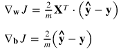
4.对每个参数,计算其对损失函数的偏导数:
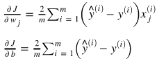
所有偏导数的梯度计算如下:
5.更新权重向量和偏置量:
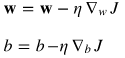
其中,![]() 表示学习率。
表示学习率。
import numpy as np
import matplotlib.pyplot as plt
'train_test_split将矩阵随机划分为训练子集和测试子集,并返回划分好的训练集测试集样本和训练集测试集标签'
from sklearn.model_selection import train_test_split
np.random.seed(123)
x = 2 * np.random.rand(500, 1)
y = 5 + 3 * x + np.random.rand(500, 1)
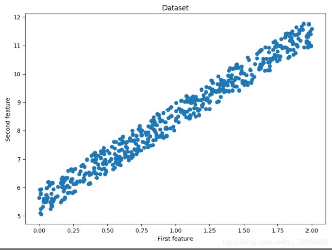
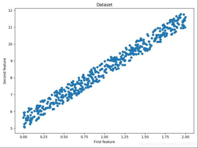
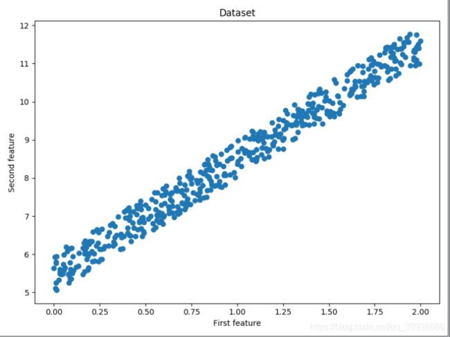
'数据集打出来看一下'
fig = plt.figure(figsize=(8,6))
plt.scatter(x, y)
plt.title('Dataset')
plt.xlabel('First feature')
plt.ylabel('Second feature')
plt.show()
x_train, x_test, y_train, y_test = train_test_split(x, y)
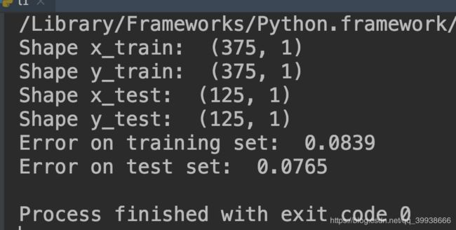
print('Shape x_train: ', x_train.shape)
print('Shape y_train: ', y_train.shape)
print('Shape x_test: ', x_test.shape)
print('Shape y_test: ', y_test.shape)
class LinearRegression:
def __init__(self):
pass
'用梯度下降方法训练'
def train_gradient_descent(self, x, y, l_r=0.01, n_iters=100):
n_samples, n_features = x.shape
self.weight = np.zeros(shape=(n_features, 1))
# print('weight: ', self.weight)
self.bias = 0
costs = []
for i in range(n_iters):
y_predict = np.dot(x, self.weight) + self.bias
cost = (1 / n_samples) * np.sum((y_predict - y)**2)
costs.append(cost)
if i % 100 == 0:
print('Cost at iteration {}:{}'.format(i, cost))
d_dw = (2 / n_samples) * np.dot(x.T, (y_predict - y))
d_db = (2 / n_samples) * np.sum((y_predict - y))
self.weight = self.weight - l_r * d_dw
self.bias = self.bias - l_r * d_db
return self.weight, self.bias, costs
def predict(self, x):
return np.dot(x, self.weight) + self.bias
regressor = LinearRegression()
w_trained, b_trained, costs = regressor.train_gradient_descent(
x_train, y_train, l_r=0.005, n_iters=600)
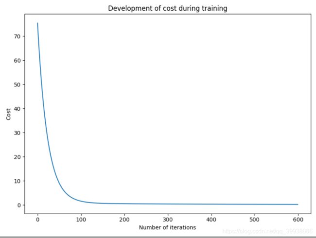
fig = plt.figure(figsize=(8,6))
plt.plot(np.arange(600), costs)
plt.title('Development of cost during training')
plt.xlabel('Number of iterations')
plt.ylabel('Cost')
plt.show()
'测试'
n_samples, _ = x_train.shape
n_samples_test, _ = x_test.shape
y_p_train = regressor.predict(x_train)
y_p_test = regressor.predict(x_test)
error_train = (1 / n_samples) * np.sum((y_p_train - y_train)**2)
error_test = (1 / n_samples_test) * np.sum((y_p_test - y_test)**2)
print('Error on training set: ', np.round(error_train, 4))
print('Error on test set: ', np.round(error_test, 4))
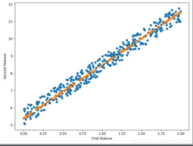
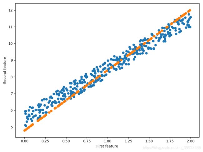
'可视化测试预测'
fig = plt.figure(figsize=(8,6))
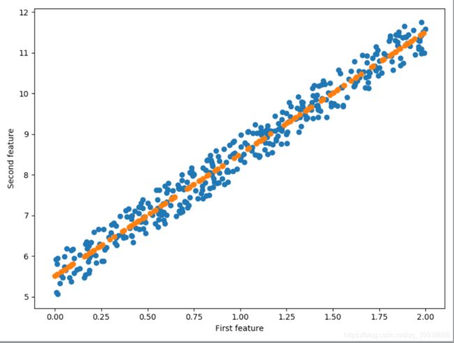
plt.scatter(x_train, y_train)
plt.scatter(x_test, y_p_test)
plt.xlabel('First feature')
plt.ylabel('Second feature')
plt.show()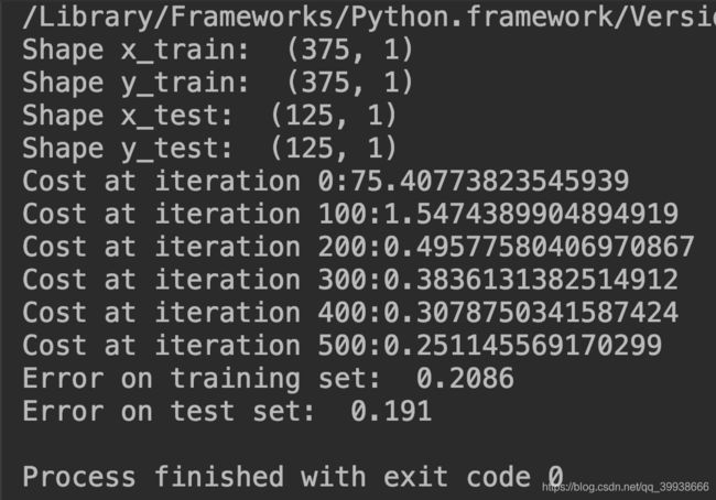
(二) 用正规方程(normal equation)训练
import numpy as np
import matplotlib.pyplot as plt
'train_test_split将矩阵随机划分为训练子集和测试子集,并返回划分好的训练集测试集样本和训练集测试集标签'
from sklearn.model_selection import train_test_split

np.random.seed(123)
x = 2 * np.random.rand(500, 1)
y = 5 + 3 * x + np.random.rand(500, 1)
'数据集打出来看一下'
fig = plt.figure(figsize=(8,6))
plt.scatter(x, y)
plt.title('Dataset')
plt.xlabel('First feature')
plt.ylabel('Second feature')
plt.show()

x_train, x_test, y_train, y_test = train_test_split(x, y)
print('Shape x_train: ', x_train.shape)
print('Shape y_train: ', y_train.shape)
print('Shape x_test: ', x_test.shape)
print('Shape y_test: ', y_test.shape)

class LinearRegression:
    def __init__(self):
        pass

    '用正规方程normal equation方法做训练'
    def train_normal_equation(self,x,y):
        self.weight = np.dot(np.dot(np.linalg.inv(np.dot(x.T, x)), x.T), y)
        self.bias = 0
        return self.weight, self.bias

    def predict(self, x):
        return np.dot(x, self.weight) + self.bias

n_samples, _ = x_train.shape
n_samples_test, _ = x_test.shape
x_b_train = np.c_[np.ones((n_samples)), x_train]#np.c_按行连接两个矩阵,把两矩阵左右相加,要求行数相等
x_b_test = np.c_[np.ones((n_samples_test)), x_test]
reg_normal = LinearRegression()
w_trained = reg_normal.train_normal_equation(x_b_train, y_train)

'测试'
y_p_train = reg_normal.predict(x_b_train)
y_p_test = reg_normal.predict(x_b_test)
error_train = (1 / n_samples) * np.sum((y_p_train - y_train)**2)
error_test = (1 / n_samples_test) * np.sum((y_p_test - y_test)**2)
print('Error on training set: ', np.round(error_train, 4))
print('Error on test set: ', np.round(error_test, 4))

'可视化测试预测'
fig = plt.figure(figsize=(8,6))
plt.scatter(x_train, y_train)
plt.scatter(x_test, y_p_test)
plt.xlabel('First feature')
plt.ylabel('Second feature')
plt.show()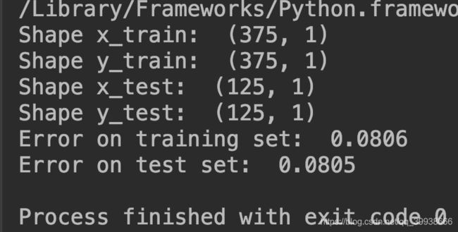
(三)直接调用sklearn的API
from sklearn.linear_model import LinearRegression         # 线性回归 #
module = LinearRegression()
module.fit(x, y)
module.score(x, y)
module.predict(test)
完整如下:
import numpy as np
import matplotlib.pyplot as plt
from sklearn.linear_model import LinearRegression#直接调用API
from sklearn.model_selection import train_test_split

np.random.seed(123)
x = 2 * np.random.rand(500, 1)
y = 5 + 3 * x + np.random.rand(500, 1)
'数据集打出来看一下'
fig = plt.figure(figsize=(8, 6))
plt.scatter(x, y)
plt.title('Dataset')
plt.xlabel('First feature')
plt.ylabel('Second feature')
plt.show()

'原始数据x,y经train_test_split处理,得到用于训练和验证的数据集x_train, x_test, y_train, y_test'
x_train, x_test, y_train, y_test = train_test_split(x, y)
print('Shape x_train: ', x_train.shape)
print('Shape y_train: ', y_train.shape)
print('Shape x_test: ', x_test.shape)
print('Shape y_test: ', y_test.shape)

module = LinearRegression()
module.fit(x_test, y_test)#fit拟合处理

'测试'
n_samples, _ = x_train.shape
n_samples_test, _ = x_test.shape
y_p_train = module.predict(x_train)
y_p_test = module.predict(x_test)
error_train = (1 / n_samples) * np.sum((y_p_train - y_train) ** 2)
error_test = (1 / n_samples_test) * np.sum((y_p_test - y_test) ** 2)
print('Error on training set: ', np.round(error_train, 4))
print('Error on test set: ', np.round(error_test, 4))

'可视化'
fig = plt.figure(figsize=(8, 6))
plt.scatter(x_train, y_train)
plt.scatter(x_test, y_p_test)
plt.xlabel('First feature')
plt.ylabel('Second feature')
plt.show()