SKlearn二分类评价指标

SKlearn的Metrics模块下有有许多二分类算法的评价指标，这里我们主要讨论最常用的几种。

1.准确度（Accuracy）

from sklearn.metrics import accuracy_score(y_true, y_pred, normalize=True, sample_weight=None)

1.1参数说明
y_true：数据的真实label值
y_pred：数据的预测标签值
normalize：默认为True，返回正确预测的个数，若是为False，返回正确预测的比例
sample_weight：样本权重
返回结果：score为正确预测的个数或者比例，由normalize确定
1.2数学表达
$$accuracy(y,\hat{y})=\frac{1}{n_{samples}}\sum _{i=0}^{n_{samples}-1}(y_i={\hat{y}}_i)$$

1.3 案列演示

import numpy as np
import pandas as pd
from sklearn.metrics import accuracy_score

y_true = [1,1,0,1,0]
y_pred = [1,1,1,0,0]

score = accuracy_score(y_true,y_pred)
print(score)
0.6#正确预测的比例

score1 = accuracy_score(y_true,y_pred,normalize = True)
print(score1)
3#正确预测的个数

2.混淆矩阵（Confusion Matrix）

from sklearn.metrics import confusion_matrix(y_true,y_pred,labels=None,sample_weight = None)

2.1参数说明
y_true：真实的label，一维数组，列名
y_pred：预测值的label，一维数组，行名
labels：默认不指定，此时y_true,y_pred去并集，做升序，做label
sample_weight：样本权重
返回结果：返回混淆矩阵
2.2案例演示

import numpy as np
from sklearn.metrics import confusion_matrix

y_true = np.array([0,1,1,1,0,0,1,2,0,1])
y_pred = np.array([0,0,1,1,1,0,1,2,0,1])

confusion_matrix = confusion_matrix(y_true,y_pred)
confusion_matrix
array([[3, 1, 0],
       [1, 4, 0],
       [0, 0, 1]], dtype=int64)

confusion_matrix的官方文档给了我们一个可将混淆矩阵可视化的模板，我们可以将模板复制过来。文档连接：https://scikit-learn.org/stable/auto_examples/model_selection/plot_confusion_matrix.html#sphx-glr-auto-examples-model-selection-plot-confusion-matrix-py

import itertools
import numpy as np
import matplotlib.pyplot as plt
from sklearn import svm, datasets
from sklearn.model_selection import train_test_split
from sklearn.metrics import confusion_matrix
def plot_confusion_matrix(cm, classes,
                          normalize=False,
                          title='Confusion matrix',
                          cmap=plt.cm.Blues):
    """
    This function prints and plots the confusion matrix.
    Normalization can be applied by setting `normalize=True`.
    """
    if normalize:
        cm = cm.astype('float') / cm.sum(axis=1)[:, np.newaxis]
        print("Normalized confusion matrix")
    else:
        print('Confusion matrix, without normalization')

    print(cm)

    plt.imshow(cm, interpolation='nearest', cmap=cmap)
    plt.title(title)
    plt.colorbar()
    tick_marks = np.arange(len(classes))
    plt.xticks(tick_marks, classes, rotation=45)
    plt.yticks(tick_marks, classes)

    fmt = '.2f' if normalize else 'd'
    thresh = cm.max() / 2.
    for i, j in itertools.product(range(cm.shape[0]), range(cm.shape[1])):
        plt.text(j, i, format(cm[i, j], fmt),
                 horizontalalignment="center",
                 color="white" if cm[i, j] > thresh else "black")

    plt.ylabel('True label')
    plt.xlabel('Predicted label')
    plt.tight_layout()

#可视化上述混淆矩阵
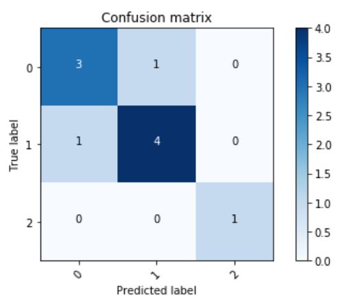
plot_confusion_matrix（confusion_matrix,classes = [0,1,2]）

如图所示，这样看上去就很直观了，中间的格子4表示1预测为1的个数有4个。

3.Precision&Recall
Precision：精确度。
Recall：召回率。
我们用一个例子来说明下Recall召回率的意思。
3.1班有100位同学，其中80位男生，20位是女生，现欲选出所有的女生，从100人中选了50人，其中20位是女生，30位是男生。
Recall中的四个指标：
TP(True positive)：预测对了，预测结果为正例（把女生预测为女生），TP = 20。
FP(False positive)：预测错了，预测结果为正例（把男生预测为女生），FP = 30。
TN(True negative)：预测对了，预测结果为负例（把男生预测为男生），TN = 50。
FN（False negative）：预测错了，预测结果为负例（把女生预测为男生），FN = 0。
Recall = TP/(TP + FN)，Recall的意思是在正确的结果中，有多少个预测结果是正确的。上述例子的Recall值就是TP/(TP+FN) = 20/(20+0) = 100%。
为什么要引入Recall这个指标呢？
假设我们现在有100个患者样本，其中有5个患者患有癌症，我们用1表示，其余95名正常患者我们用0表示。假设我们现在用一种算法做预测，所有的结果都预测为0，95个肯定是预测对了，算法准确率为95%，看着挺高的。但是这个算法对于癌症患者的预测准确率是0，所以这个算法是没有任何意义的。这时候我们的recall值的价值就体现出来了，recall值是在5个癌症患者中找能预测出来的，如果预测3个对了，recall = 60%。

from sklearn.metrics import classification_report(y_true, y_pred, labels=None, 
target_names=None, sample_weight=None, digits=2, output_dict=False)

3.1参数说明
y_true：真实的label，一维数组，列名
y_pred：预测值的label，一维数组，行名
labels：默认不指定，此时y_true,y_pred去并集，做升序，做label
sample_weight：样本权重
target_names：行标签，顺序和label的要一致
digits，整型，小数的位数
out_dict：输出格式，默认False，如果为True，输出字典。
3.2样例演示

import numpy as np
from sklearn.metrics import classification_report

y_true = np.array([0,1,1,0,1,2,1])
y_pred = np.array([0,1,0,0,1,2,1])
target_names = ['class0','class1','class2']
print(classification_report(y_true,y_pred,target_names = target_names))
#结果如下
  precision    recall  f1-score   support

      class0       0.67      1.00      0.80         2
      class1       1.00      0.75      0.86         4
      class2       1.00      1.00      1.00         1

   micro avg       0.86      0.86      0.86         7
   macro avg       0.89      0.92      0.89         7
weighted avg       0.90      0.86      0.86         7

补充：f1-score是recall与precision的综合结果，其表达式为：f1-score = 2 * (precision * recall)/(precision + recall)
4.ROC_AUC

from sklearn.metrics import roc_auc_score(y_true, y_score, average=’macro’, 
sample_weight=None, max_fpr=None)

4.1参数说明
y_true：真实的label，一维数组
y_score：模型预测的正例的概率值
average：有多个参数可选，一般默认即可
sample_weight：样本权重
max_fpr 取值范围[0，1),如果不是None，则会标准化，使得最大值=max_fpr
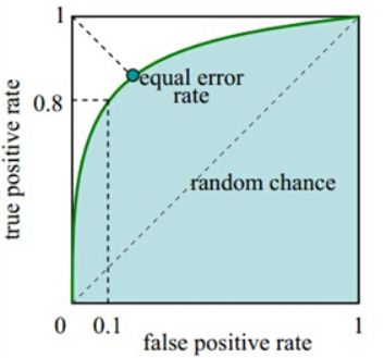
4.2 Roc曲线说明
如下图所示，横轴表示false positive rate，纵轴表示true positive rate，我们希望false positive rate的值越小越好，true positive rate的值越大越好，希望曲线往左上角偏。那么如何衡量Roc曲线，我们用Roc的曲线面积来衡量即Auc（Area under curve）值，取值范围：[0,1]。

4.3样例演示

import numpy as np
from sklearn.metrics import roc_auc_score

y_true = np.array([0,1,1,0])
y_score = np.array([0.85,0.78,0.69,0.54])
print(roc_auc_score(y_true,y_score))
0.5

5.小结
评估机器学习算法是我们在解决实际问题中非常重要的一步，只有通过准确的评估，我们才能对算法进行后期的优化处理。这一节所说的Precision,Recall,Confusion_matrix,Roc_Auc是我们最常用的二分类算法的评估方法。以后在解决实际问题时，单一的评估指标往往不能反映出真正的算法效果，所以我们需综合多种评估指标来评价某一种算法。