二手车交易价格实战

一.赛题理解

1.1赛题材料

赛题：零基础入门数据挖掘 - 二手车交易价格预测

链接：https://tianchi.aliyun.com/competition/entrance/231784/introduction?spm=5176.12281957.1004.1.38b02448ausjSX

问题：赛题以二手车市场为背景，要求选手预测二手汽车的交易价格，这是一个典型的回归问题。

数据：该数据来自某交易平台的二手车交易记录，总数据量超过40w，包含31列变量信息，其中15列为匿名变量。为了保证比赛的公平性，将会从中抽取15万条作为训练集，5万条作为测试集A，5万条作为测试集B，同时会对name、model、brand和regionCode等信息进行脱敏。

评价标准：评价标准为MAE(Mean Absolute Error)。
enter image description here
MAE越小，说明模型预测得越准确。

1.2分析

1.此题为传统的数据挖掘问题，通过数据科学以及机器学习深度学习的办法来进行建模得到结果。
2.此题是一个典型的回归问题。
3.主要应用xgb、lgb、catboost，以及pandas、numpy、matplotlib、seabon、sklearn、keras等等数据挖掘常用库或者框架来进行数据挖掘任务。
4.通过EDA来挖掘数据的联系和自我熟悉数据。

二、 EDA-数据探索性分析

EDA (Exploratory Data Analysis)，即对数据进行探索性的分析。在数据清洗和特征工程之前，通过作图，制表等方式对数据进行特征（统计性特征，分布型特征，相关性）分析。

当了解了数据集之后我们下一步就是要去了解变量间的相互关系以及变量与预测值之间的存在关系。

引导数据科学从业者进行数据处理以及特征工程的步骤,使数据集的结构和特征集让接下来的预测问题更加可靠。

完成对于数据的探索性分析，并对于数据进行一些图表或者文字总结并打卡。

前期准备：导入所需的包

import numpy as np
import pandas as pd
import matplotlib.pyplot as plt
import seaborn as sns
import missingno as msno

numpy:Python科学计算库，主要功能之一是用来操作数组和矩阵.

pandas:提供了大量能使我们快速便捷地处理数据的函数和方法.

matplotlib:可视化

seaborn：基于matplotlib的图形可视化python包，提供了一种高度交互式界面，便于用户能够做出各种有吸引力的统计图表.

missingno：缺失值可视化

2.1加载数据

Train_data=pd.read_csv('E:\Train_data.csv',sep=' ')
Test_data=pd.read_csv('E:\Test_data.csv',sep=' ')

pandas加载与数据预处理：https://blog.csdn.net/weixin_43697287/article/details/86365049

2.2数据概括

#数据大小（行数与列数）
print('Train_data.shape:',Train_data.shape)
print('Test_data.shape:',Test_data.shape)

Train_data.shape: (150000, 31)
Test_data.shape: (50000, 30)

#索引，数据类型和内存信息
print('Train_data.info:',Train_data.info())
print('Test_data.info:',Test_data.info())

RangeIndex: 150000 entries, 0 to 149999
Data columns (total 31 columns):
SaleID               150000 non-null int64
name                 150000 non-null int64
regDate              150000 non-null int64
model                149999 non-null float64
brand                150000 non-null int64
bodyType             145494 non-null float64
fuelType             141320 non-null float64
gearbox              144019 non-null float64
power                150000 non-null int64
kilometer            150000 non-null float64
notRepairedDamage    150000 non-null object
regionCode           150000 non-null int64
seller               150000 non-null int64
offerType            150000 non-null int64
creatDate            150000 non-null int64
price                150000 non-null int64
v_0                  150000 non-null float64
v_1                  150000 non-null float64
v_2                  150000 non-null float64
v_3                  150000 non-null float64
v_4                  150000 non-null float64
v_5                  150000 non-null float64
v_6                  150000 non-null float64
v_7                  150000 non-null float64
v_8                  150000 non-null float64
v_9                  150000 non-null float64
v_10                 150000 non-null float64
v_11                 150000 non-null float64
v_12                 150000 non-null float64
v_13                 150000 non-null float64
v_14                 150000 non-null float64
dtypes: float64(20), int64(10), object(1)
memory usage: 35.5+ MB
Train_data.info: None

RangeIndex: 50000 entries, 0 to 49999
Data columns (total 30 columns):
SaleID               50000 non-null int64
name                 50000 non-null int64
regDate              50000 non-null int64
model                50000 non-null float64
brand                50000 non-null int64
bodyType             48587 non-null float64
fuelType             47107 non-null float64
gearbox              48090 non-null float64
power                50000 non-null int64
kilometer            50000 non-null float64
notRepairedDamage    50000 non-null object
regionCode           50000 non-null int64
seller               50000 non-null int64
offerType            50000 non-null int64
creatDate            50000 non-null int64
v_0                  50000 non-null float64
v_1                  50000 non-null float64
v_2                  50000 non-null float64
v_3                  50000 non-null float64
v_4                  50000 non-null float64
v_5                  50000 non-null float64
v_6                  50000 non-null float64
v_7                  50000 non-null float64
v_8                  50000 non-null float64
v_9                  50000 non-null float64
v_10                 50000 non-null float64
v_11                 50000 non-null float64
v_12                 50000 non-null float64
v_13                 50000 non-null float64
v_14                 50000 non-null float64
dtypes: float64(20), int64(9), object(1)
memory usage: 11.4+ MB
Test_data.info: None

2.3数据缺失与异常

2.3.1分析数据

analyze= []
for col in Train_data.columns:
    analyze.append((col, Train_data[col].nunique(), Train_data[col].isnull().sum() * 100 / Train_data.shape[0],Train_data[col].value_counts(normalize=True, dropna=False).values[0] * 100, Train_data[col].dtype))
analyze_df = pd.DataFrame(analyze, columns=['Feature', 'Unique_values', 'Percentage of missing values','Percentage of values in the biggest category', 'type'])
analyze_df.sort_values('Percentage of missing values', ascending=False, inplace=True)
analyze_df

	Feature	Unique_values	Percentage of missing values	Percentage of values in the biggest category	type
6	fuelType	7	5.786667	61.104000	float64
7	gearbox	2	3.987333	74.415333	float64
5	bodyType	8	3.004000	27.613333	float64
3	model	248	0.000667	7.841333	float64
0	SaleID	150000	0.000000	0.000667	int64
24	v_8	142451	0.000000	1.064667	float64
20	v_4	143998	0.000000	0.013333	float64
21	v_5	139624	0.000000	2.990000	float64
22	v_6	109766	0.000000	23.643333	float64
23	v_7	138709	0.000000	3.644667	float64
27	v_11	143997	0.000000	0.013333	float64
25	v_9	140617	0.000000	2.324000	float64
26	v_10	143997	0.000000	0.013333	float64
18	v_2	143997	0.000000	0.013333	float64
28	v_12	143997	0.000000	0.013333	float64
29	v_13	143998	0.000000	0.013333	float64
19	v_3	143998	0.000000	0.013333	float64
15	price	3763	0.000000	1.558000	int64
17	v_1	143998	0.000000	0.013333	float64
16	v_0	143997	0.000000	0.013333	float64
1	name	99662	0.000000	0.188000	int64
14	creatDate	96	0.000000	3.898667	int64
13	offerType	1	0.000000	100.000000	int64
12	seller	2	0.000000	99.999333	int64
11	regionCode	7905	0.000000	0.246000	int64
10	notRepairedDamage	3	0.000000	74.240667	object
9	kilometer	13	0.000000	64.584667	float64
8	power	566	0.000000	8.552667	int64
4	brand	40	0.000000	20.986667	int64
2	regDate	3894	0.000000	0.120000	int64
30	v_14	143998	0.000000	0.013333	float64

nunique() 方法用于获取 'Team’列中所有唯一值的数量。

观察上图可发现发现价格、功率、行驶里程有0值，在实际中是很不现实的，后续需分析是异常还是脱敏后的正常值。

只有notRepairedDamage的格式为object。
notRepairedDamage在赛题中说明只有0和1两类，统计却出现3类。
offerType在赛题中说明有0和1两类，统计只有1类。 seller2类中有1大类占据极大部分（百分之99多），存在严重的倾斜。

2.3.2缺失与异常处理

异常处理

Train_data['notRepairedDamage'].value_counts()

0.0    111361
-       24324
1.0     14315
Name: notRepairedDamage, dtype: int64

Test_data['notRepairedDamage'].value_counts()

0.0    37249
-       8031
1.0     4720
Name: notRepairedDamage, dtype: int64

经上述的展开，发现notRepairedDamage里有空格，故将其分为了三类。因为很多模型对nan有直接的处理，这里我们先不做处理，先替换成nan

Train_data['notRepairedDamage'].replace('-', np.nan, inplace=True)
Test_data['notRepairedDamage'].replace('-', np.nan, inplace=True)

Train_data['notRepairedDamage'].value_counts()

0.0    111361
1.0     14315
Name: notRepairedDamage, dtype: int64

offerType，seller两个字段对价格影响特别小，可删除

del Train_data["seller"]
del Train_data["offerType"]
del Test_data["seller"]
del Test_data["offerType"]

缺失处理

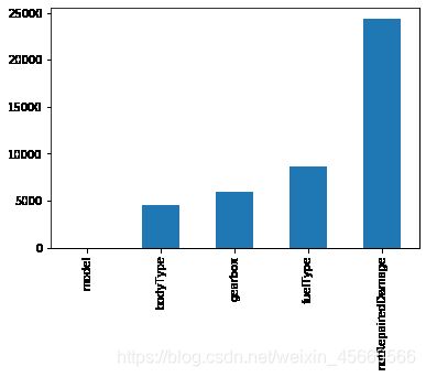
# 缺失值可视化
missing = Train_data.isnull().sum()
missing = missing[missing > 0]#获取空值>0的列
missing.sort_values(inplace=True)#排序
missing.plot.bar()

msno.matrix(Train_data.sample(250))#msno矩阵查看缺失值

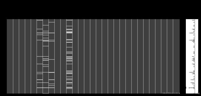
msno.bar(Train_data.sample(1000))#msno 条形图查看缺失值

缺失值可视化后可以发现bodyType、fuelType、gearbox缺失值比较多，后续需要对这些字段缺失值进行处理

2.4预测值分布

Train_data['price']

0         1850
1         3600
2         6222
3         2400
4         5200
          ... 
149995    5900
149996    9500
149997    7500
149998    4999
149999    4700
Name: price, Length: 150000, dtype: int64

Train_data['price'].value_counts()

500      2337
1500     2158
1200     1922
1000     1850
2500     1821
         ... 
25321       1
8886        1
8801        1
37920       1
8188        1
Name: price, Length: 3763, dtype: int64

## 1) 价格总体分布概况
import scipy.stats as st
y = Train_data['price']
plt.figure(1); plt.title('Johnson SU')
sns.distplot(y, kde=False, fit=st.johnsonsu)
plt.figure(2); plt.title('Normal')
sns.distplot(y, kde=False, fit=st.norm)
plt.figure(3); plt.title('Log Normal')
sns.distplot(y, kde=False, fit=st.lognorm)

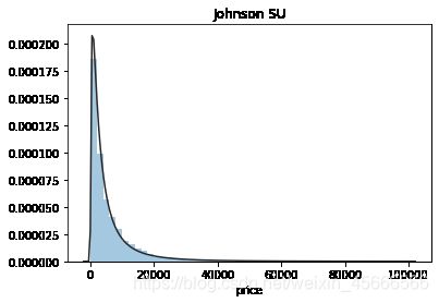
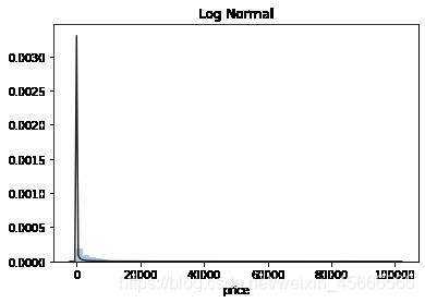
观察总体分布，发现Johnson SU拟合效果较好，价格数据分布存在右偏，说明存在过大的极端值。

查看数据的偏度和峰度
skew、kurt说明参考https://www.cnblogs.com/wyy1480/p/10474046.html

#查看skewness and kurtosis
sns.distplot(Train_data['price']);
print("Skewness: %f" % Train_data['price'].skew())
print("Kurtosis: %f" % Train_data['price'].kurt())

Skewness: 3.346487
Kurtosis: 18.995183

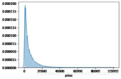
从偏度值大于0也可得知数据右偏。从价格分布中可以看出价格大于40000后的二手车数量极少。

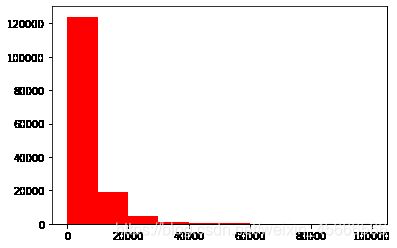
#查看预测值的具体频数
plt.hist(Train_data['price'], orientation = 'vertical',histtype = 'bar', color ='red')

(array([1.23906e+05, 1.89270e+04, 4.91800e+03, 1.34000e+03, 4.71000e+02,
        1.88000e+02, 1.24000e+02, 6.00000e+01, 4.80000e+01, 1.80000e+01]),
 array([1.10000e+01, 1.00098e+04, 2.00086e+04, 3.00074e+04, 4.00062e+04,
        5.00050e+04, 6.00038e+04, 7.00026e+04, 8.00014e+04, 9.00002e+04,
        9.99990e+04]),
 )

#查看预测值的箱型图
Train_data['price'].plot(kind='box')

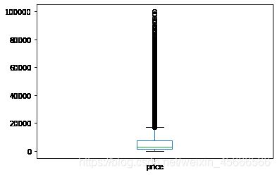
再利用箱型图，频数图查看具体的分布划分，看出价格大于20000则为异常值。

将价格大于20000的数据剔除，再重新画图

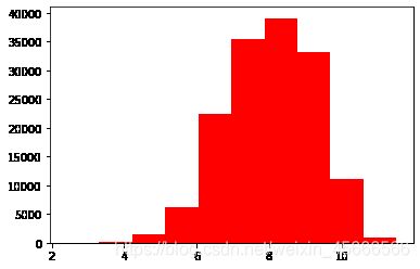
Train_data[Train_data['price']<=20000]['price'].hist()

# log变换 z之后的分布较均匀，可以进行log变换进行预测，这也是预测问题常用的trick
plt.hist(np.log(Train_data['price']), orientation = 'vertical',histtype = 'bar', color ='red') 
plt.show()

2.5特征分析

特征数据分为定类数据、定序数据、定距数据、定比数据四类，需要分别分析。

在本次赛题中提供的数据类型有定类数据和定距数据。

numeric_features = ['power', 'kilometer', 'v_0', 'v_1', 'v_2', 'v_3', 'v_4', 'v_5', 'v_6', 'v_7', 'v_8', 'v_9', 'v_10', 'v_11', 'v_12', 'v_13','v_14' ]

categorical_features = ['name', 'model', 'brand', 'bodyType', 'fuelType', 'gearbox', 'notRepairedDamage', 'regionCode',]

2.5.1数字特征分析

numeric_features.append('price')#添加price特征

## 1) 相关性分析
numeric_feature_price=Train_data[numeric_features]
colormap = plt.cm.magma
plt.figure(figsize=(16,14))
plt.title('Pearson correlation of continuous features', y=1.05, size=15)
sns.heatmap(numeric_feature_price.corr(),linewidths=0.1,vmax=1.0, square=True, 
            cmap=colormap, linecolor='white', annot=True)

correction=numeric_feature_price.corr()

print(correlation['price'].sort_values(ascending = False),'\n')

price        1.000000
v_12         0.692823
v_8          0.685798
v_0          0.628397
power        0.219834
v_5          0.164317
v_2          0.085322
v_6          0.068970
v_1          0.060914
v_14         0.035911
v_13        -0.013993
v_7         -0.053024
v_4         -0.147085
v_9         -0.206205
v_10        -0.246175
v_11        -0.275320
kilometer   -0.440519
v_3         -0.730946
Name: price, dtype: float64 

从相关性图表中，可以看到不同定距数据之间的相关性大小。
从中可挑选出与价格相关性较大的特征，剔除相关性为0的特征。
此外回归预测中需要解决共线性特征。v_6与v_1相关性为1，需判断是否为重复列。此外v0-v14的大部分特征的相关性系数比较大，需要进行降维处理。

## 2) 查看几个特征得 偏度和峰值
for col in numeric_features:
    print('{:15}'.format(col), 
          'Skewness: {:05.2f}'.format(Train_data[col].skew()) , 
          '   ' ,
          'Kurtosis: {:06.2f}'.format(Train_data[col].kurt())  
         )

power           Skewness: 65.86     Kurtosis: 5733.45
kilometer       Skewness: -1.53     Kurtosis: 001.14
v_0             Skewness: -1.32     Kurtosis: 003.99
v_1             Skewness: 00.36     Kurtosis: -01.75
v_2             Skewness: 04.84     Kurtosis: 023.86
v_3             Skewness: 00.11     Kurtosis: -00.42
v_4             Skewness: 00.37     Kurtosis: -00.20
v_5             Skewness: -4.74     Kurtosis: 022.93
v_6             Skewness: 00.37     Kurtosis: -01.74
v_7             Skewness: 05.13     Kurtosis: 025.85
v_8             Skewness: 00.20     Kurtosis: -00.64
v_9             Skewness: 00.42     Kurtosis: -00.32
v_10            Skewness: 00.03     Kurtosis: -00.58
v_11            Skewness: 03.03     Kurtosis: 012.57
v_12            Skewness: 00.37     Kurtosis: 000.27
v_13            Skewness: 00.27     Kurtosis: -00.44
v_14            Skewness: -1.19     Kurtosis: 002.39
price           Skewness: 03.35     Kurtosis: 019.00

## 3) 每个数字特征得分布可视化
f = pd.melt(Train_data, value_vars=numeric_features)
g = sns.FacetGrid(f, col="variable",  col_wrap=2, sharex=False, sharey=False)
g = g.map(sns.distplot, "value")

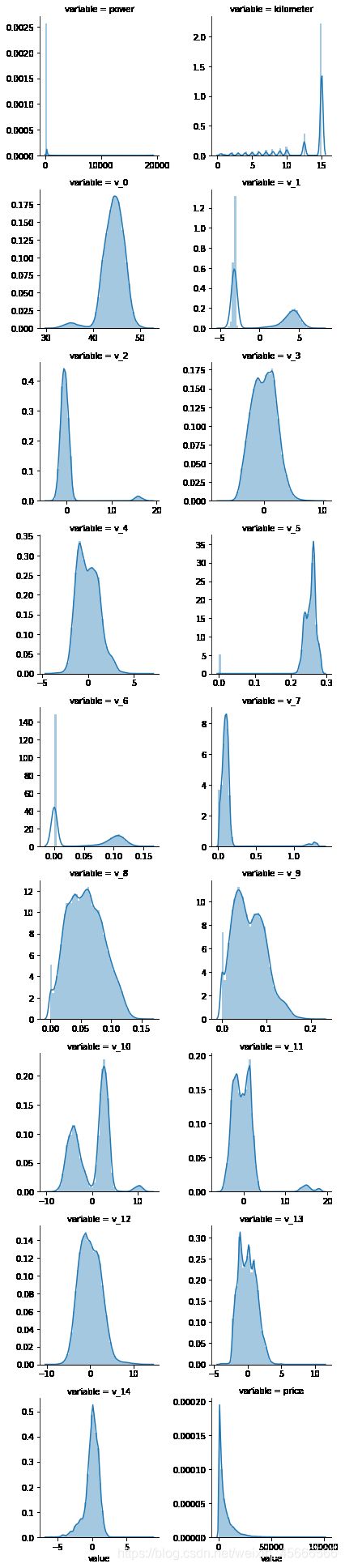
v0-v4的特征分布相对均匀。而power的偏度和峰度特别大，右偏且特别峰顶尖锐。因此，需具体查看power的数据分布。

plt.figure(figsize=[16,4])
plt.subplot(1,2,1)
Train_data['power'].plot(kind='box')
plt.subplot(1,2,2)
Train_data['power'].hist()

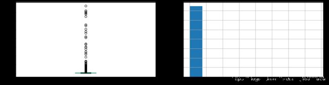
从power的箱型图和直方图中可以看到，power大于2500的二手车数量非常少，
将power大于2500的数据剔除继续画图，发现仍然存在异常的值，结合赛题的字段说明中，
power的范围为[0,600]，因此，将power大于600的剔除，继续画图观察。
并将power进行log转换，发现数据有2部分。左边为0的同样是异常值，汽车功率不可能为0。因此，后续将对power大于600及为0的值进行异常值处理，
并对power进行log转换。

plt.figure(figsize=[16,4])
plt.subplot(1,2,1)
Train_data[Train_data['power']<=2500]['power'].plot(kind='box')
plt.subplot(1,2,2)
Train_data[Train_data['power']<=2500]['power'].hist()

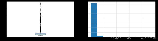
plt.figure(figsize=[16,4])
plt.subplot(1,3,1)
Train_data[Train_data['power']<=600]['power'].plot(kind='box')
plt.subplot(1,3,2)
Train_data[Train_data['power']<=600]['power'].hist()
plt.subplot(1,3,3)
np.log(Train_data[Train_data['power']<=600]['power']+1).hist()

## 4) 数字特征相互之间的关系可视化
sns.set()
columns = ['price', 'v_12', 'v_8' , 'v_0', 'power', 'v_5',  'v_2', 'v_6', 'v_1', 'v_14']
sns.pairplot(Train_data[columns],height = 2 ,kind ='scatter',diag_kind='kde')
plt.show()

Y_train = Train_data['price']

## 5) 多变量互相回归关系可视化
fig, ((ax1, ax2), (ax3, ax4), (ax5, ax6), (ax7, ax8), (ax9, ax10)) = plt.subplots(nrows=5, ncols=2, figsize=(24, 20))
# ['v_12', 'v_8' , 'v_0', 'power', 'v_5',  'v_2', 'v_6', 'v_1', 'v_14']
v_12_scatter_plot = pd.concat([Y_train,Train_data['v_12']],axis = 1)
sns.regplot(x='v_12',y = 'price', data = v_12_scatter_plot,scatter= True, fit_reg=True, ax=ax1)

v_8_scatter_plot = pd.concat([Y_train,Train_data['v_8']],axis = 1)
sns.regplot(x='v_8',y = 'price',data = v_8_scatter_plot,scatter= True, fit_reg=True, ax=ax2)

v_0_scatter_plot = pd.concat([Y_train,Train_data['v_0']],axis = 1)
sns.regplot(x='v_0',y = 'price',data = v_0_scatter_plot,scatter= True, fit_reg=True, ax=ax3)

power_scatter_plot = pd.concat([Y_train,Train_data['power']],axis = 1)
sns.regplot(x='power',y = 'price',data = power_scatter_plot,scatter= True, fit_reg=True, ax=ax4)

v_5_scatter_plot = pd.concat([Y_train,Train_data['v_5']],axis = 1)
sns.regplot(x='v_5',y = 'price',data = v_5_scatter_plot,scatter= True, fit_reg=True, ax=ax5)

v_2_scatter_plot = pd.concat([Y_train,Train_data['v_2']],axis = 1)
sns.regplot(x='v_2',y = 'price',data = v_2_scatter_plot,scatter= True, fit_reg=True, ax=ax6)

v_6_scatter_plot = pd.concat([Y_train,Train_data['v_6']],axis = 1)
sns.regplot(x='v_6',y = 'price',data = v_6_scatter_plot,scatter= True, fit_reg=True, ax=ax7)

v_1_scatter_plot = pd.concat([Y_train,Train_data['v_1']],axis = 1)
sns.regplot(x='v_1',y = 'price',data = v_1_scatter_plot,scatter= True, fit_reg=True, ax=ax8)

v_14_scatter_plot = pd.concat([Y_train,Train_data['v_14']],axis = 1)
sns.regplot(x='v_14',y = 'price',data = v_14_scatter_plot,scatter= True, fit_reg=True, ax=ax9)

v_13_scatter_plot = pd.concat([Y_train,Train_data['v_13']],axis = 1)
sns.regplot(x='v_13',y = 'price',data = v_13_scatter_plot,scatter= True, fit_reg=True, ax=ax10)

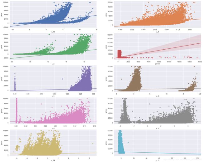
此处是多变量之间的关系可视化，
可视化更多学习可参考很不错的文章 https://www.jianshu.com/p/6e18d21a4cad¶

2.5.2类别特征分析

## 1) unique分布
for fea in categorical_features:
    print(Train_data[fea].nunique())

99662
248
40
8
7
2
2
7905

categorical_features

['name',
 'model',
 'brand',
 'bodyType',
 'fuelType',
 'gearbox',
 'notRepairedDamage',
 'regionCode']

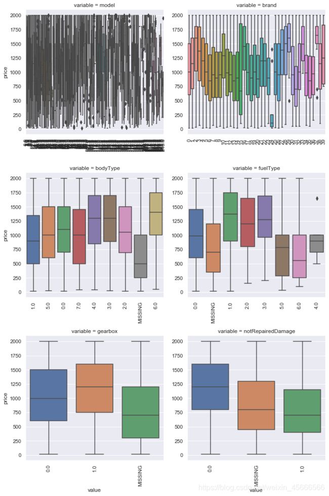
## 2) 类别特征箱形图可视化

# 因为 name和 regionCode的类别太稀疏了，这里我们把不稀疏的几类画一下
categorical_features = ['model',
 'brand',
 'bodyType',
 'fuelType',
 'gearbox',
 'notRepairedDamage']
for c in categorical_features:
    Train_data[c] = Train_data[c].astype('category')
    if Train_data[c].isnull().any():
        Train_data[c] = Train_data[c].cat.add_categories(['MISSING'])
        Train_data[c] = Train_data[c].fillna('MISSING')

def boxplot(x, y, **kwargs):
    sns.boxplot(x=x, y=y)
    x=plt.xticks(rotation=90)

f = pd.melt(Train_data[Train_data['price']<=2000], id_vars=['price'], value_vars=categorical_features)
g = sns.FacetGrid(f, col="variable",  col_wrap=2, sharex=False, sharey=False, height=5)
g = g.map(boxplot, "value", "price")

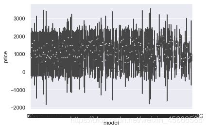
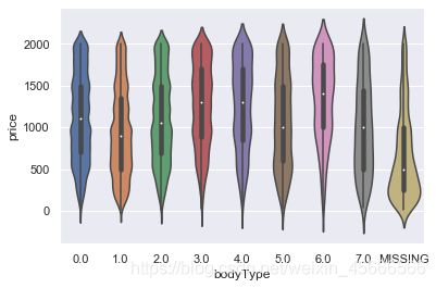
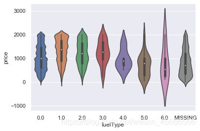
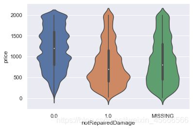
## 3) 类别特征的小提琴图可视化
catg_list = categorical_features
target = 'price'
for catg in catg_list :
    sns.violinplot(x=catg, y=target, data=Train_data[Train_data['price']<=2000])
    plt.show()

分析日期与价格关系

df_Train=Train_data.loc[:,['regDate','creatDate','price']]
#转换日期格式
df_Train['regDate']=df_Train['regDate'].astype(str)
df_Train['creatDate']=df_Train['creatDate'].astype(str)
df_Train['regyear']=df_Train['regDate'].str[0:4]
df_Train['creatyear']=df_Train['creatDate'].str[0:4]
df_Train['regmonth']=df_Train['regDate'].str[4:6]
df_Train['creatmonth']=df_Train['creatDate'].str[4:6]

df_Train['creatyear'].value_counts()

2016    149982
2015        18
Name: creatyear, dtype: int64

用pandas_profiling生成数据报告

用pandas_profiling生成一个较为全面的可视化和数据报告(较为简单、方便) 最终打开html文件即可

#import pandas_profiling
#pfr = pandas_profiling.ProfileReport(Train_data)
#pfr.to_file("./example.html")

三.总结

1. 所给出的EDA步骤为广为普遍的步骤，在实际的不管是工程还是比赛过程中，这只是最开始的一步，也是最基本的一步。
2. 接下来一般要结合模型的效果以及特征工程等来分析数据的实际建模情况，根据自己的一些理解，查阅文献，对实际问题做出判断和深入的理解。
3. 最后不断进行EDA与数据处理和挖掘，来到达更好的数据结构和分布以及较为强势相关的特征

参考资料：
https://tianchi.aliyun.com/notebook-ai/detail?postId=95457