聚类Clustering
十三、聚类
1. 样本相似性:欧氏距离
- 用两个样本对应特征值之差的平方和之平方根,即欧氏距离,来表示这两个样本的相似性。
P ( x 1 ) − Q ( x 2 ) : ∣ x 1 − x 2 ∣ = ( x 1 − x 2 ) 2 P(x1)-Q(x2):|x1-x2|=\sqrt{(x1-x2)^2} P(x1)−Q(x2):∣x1−x2∣=(x1−x2)2
P ( x 1 , y 1 ) − Q ( x 2 , y 2 ) : ( x 1 − x 2 ) 2 + ( y 1 − y 2 ) 2 P(x1,y1)-Q(x2,y2):\sqrt{(x1-x2)^2+(y1-y2)^2} P(x1,y1)−Q(x2,y2):(x1−x2)2+(y1−y2)2
P ( x 1 , y 1 , z 1 ) − Q ( x 2 , y 2 , z 2 ) : ( x 1 − x 2 ) 2 + ( y 1 − y 2 ) 2 + ( z 1 − z 2 ) 2 P(x1,y1,z1)-Q(x2,y2,z2): \sqrt{(x1-x2)^2+(y1-y2)^2+(z1-z2)^2} P(x1,y1,z1)−Q(x2,y2,z2):(x1−x2)2+(y1−y2)2+(z1−z2)2
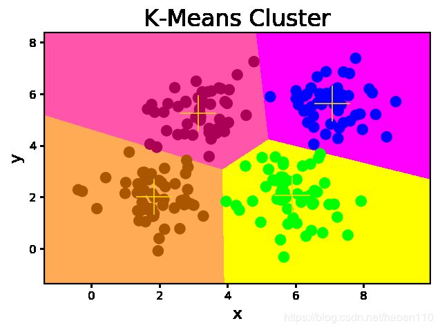
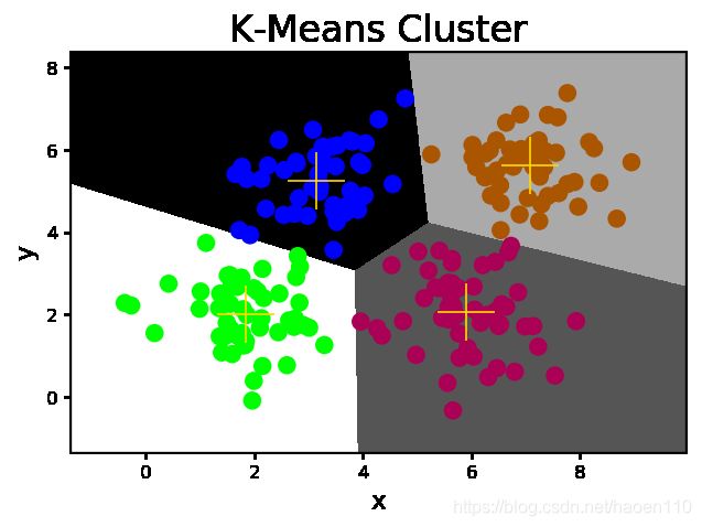
2. K均值算法
-
第一步:随机选择k个样本作为k个聚类的中心,计算每个样本到各个聚类中心的欧氏距离,将该样本分配到与之距离最近的聚类中心所在的类别中。
-
第二步:根据第一步所得到的聚类划分,分别计算每个聚类的几何中心,将几何中心作为新的聚类中心,重复第一步,直到计算所得几何中心与聚类中心重合或接近重合为止。
- 聚类数k必须事先已知。借助某些评估指标,优选最好的聚类数。
- 聚类中心的初始选择会影响到最终聚类划分的结果。初始中心尽量选择距离较远的样本。
# km.py
import numpy as np
import sklearn.cluster as sc
import matplotlib.pyplot as mp
x = []
with open('../data/multiple3.txt', 'r') as f:
    for line in f.readlines():
        data = [float(substr) for substr in line.split(',')]
        x.append(data)
x = np.array(x)

# K均值聚类器
model = sc.KMeans(n_clusters=4)
model.fit(x)
centers = model.cluster_centers_
l, r, h = x[:, 0].min() - 1, x[:, 0].max() + 1, 0.005
b, t, v = x[:, 1].min() - 1, x[:, 1].max() + 1, 0.005
grid_x = np.meshgrid(np.arange(l, r, h), np.arange(b, t, v))
flat_x = np.c_[grid_x[0].ravel(), grid_x[1].ravel()]
flat_y = model.predict(flat_x)
grid_y = flat_y.reshape(grid_x[0].shape)
pred_y = model.predict(x)
mp.figure('K-Means Cluster', dpi=120)
mp.title('K-Means Cluster', fontsize=20)
mp.xlabel('x', fontsize=14)
mp.ylabel('y', fontsize=14)
mp.tick_params(labelsize=10)
mp.pcolormesh(grid_x[0], grid_x[1], grid_y, cmap='spring')
mp.scatter(x[:, 0], x[:, 1], c=pred_y, cmap='brg', s=80)
mp.scatter(centers[:, 0], centers[:, 1], marker='+', c='gold', s=1000, linewidth=1)
mp.show()
# quant.py
import numpy as np
import scipy.misc as sm
import scipy.ndimage as sn
import sklearn.cluster as sc
import matplotlib.pyplot as mp
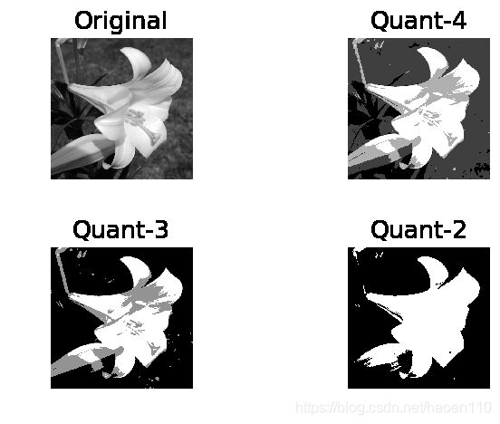
# 通过K均值聚类量化图像中的颜色
def quant(image, n_clusters):
x = image.reshape(-1, 1)
model = sc.KMeans(n_clusters=n_clusters)
model.fit(x)
y = model.labels_
centers = model.cluster_centers_.squeeze()
return centers[y].reshape(image.shape)
original = sm.imread('../data/lily.jpg', True)
quant4 = quant(original, 4)
quant3 = quant(original, 3)
quant2 = quant(original, 2)
mp.figure('Image Quant', dpi=120)
mp.subplot(221)
mp.title('Original', fontsize=16)
mp.axis('off')
mp.imshow(original, cmap='gray')
mp.subplot(222)
mp.title('Quant-4', fontsize=16)
mp.axis('off')
mp.imshow(quant4, cmap='gray')
mp.subplot(223)
mp.title('Quant-3', fontsize=16)
mp.axis('off')
mp.imshow(quant3, cmap='gray')
mp.subplot(224)
mp.title('Quant-2', fontsize=16)
mp.axis('off')
mp.imshow(quant2, cmap='gray')
mp.tight_layout()
mp.show()
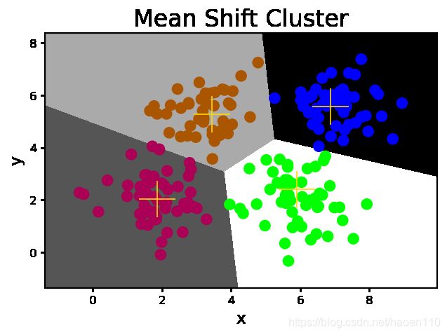
3. 均值漂移算法
-
首先假定样本空间中的每个聚类均服从某种已知的概率分布规则,然后用不同的概率密度函数拟合样本中的统计直方图,不断移动密度函数的中心(均值)的位置,直到获得最佳拟合效果为止。这些概率密度函数的峰值点就是聚类的中心,再根据每个样本距离各个中心的距离,选择最近聚类中心所属的类别作为该样本的类别。
- 聚类数不必事先已知,算法会自动识别出统计直方图的中心数量。
- 聚类中心不依据于最初假定,聚类划分的结果相对稳定。
- 样本空间应该服从某种概率分布规则,否则算法的准确性会大打折扣。
# shift.py
import numpy as np
import sklearn.cluster as sc
import matplotlib.pyplot as mp
x = []
with open('../data/multiple3.txt', 'r') as f:
    for line in f.readlines():
        data = [float(substr) for substr in line.split(',')]
        x.append(data)
x = np.array(x)

# 量化带宽,决定每次调整概率密度函数的步进量
bw = sc.estimate_bandwidth(x, n_samples=len(x), quantile=0.1)

# 均值漂移聚类器
model = sc.MeanShift(bandwidth=bw, bin_seeding=True)
model.fit(x)
centers = model.cluster_centers_
l, r, h = x[:, 0].min() - 1, x[:, 0].max() + 1, 0.005
b, t, v = x[:, 1].min() - 1, x[:, 1].max() + 1, 0.005
grid_x = np.meshgrid(np.arange(l, r, h), np.arange(b, t, v))
flat_x = np.c_[grid_x[0].ravel(), grid_x[1].ravel()]
flat_y = model.predict(flat_x)
grid_y = flat_y.reshape(grid_x[0].shape)
pred_y = model.predict(x)
mp.figure('Mean Shift Cluster', dpi=120)
mp.title('Mean Shift Cluster', fontsize=20)
mp.xlabel('x', fontsize=14)
mp.ylabel('y', fontsize=14)
mp.tick_params(labelsize=10)
mp.pcolormesh(grid_x[0], grid_x[1], grid_y, cmap='gray')
mp.scatter(x[:, 0], x[:, 1], c=pred_y, cmap='brg', s=80)
mp.scatter(centers[:, 0], centers[:, 1], marker='+', c='gold', s=1000, linewidth=1)
mp.show()
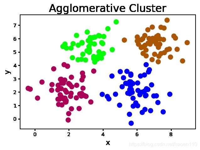
4. 凝聚层次算法
-
首先假定每个样本都是一个独立的聚类,如果统计出来的聚类数大于期望的聚类数,则从每个样本出发寻找离自己最近的另一个样本,与之聚集,形成更大的聚类,同时令总聚类数减少,不断重复以上过程,直到统计出来的聚类数达到期望值为止。
- 聚类数k必须事先已知。借助某些评估指标,优选最好的聚类数。
- 没有聚类中心的概念,因此只能在训练集中划分聚类,但不能对训练集以外的未知样本确定其聚类归属。
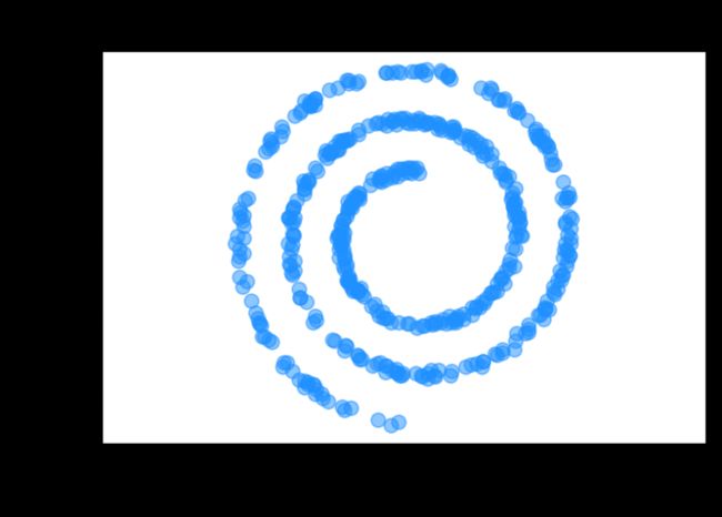
- 在确定被凝聚的样本时,除了以距离作为条件以外,还可以根据连续性来确定被聚集的样本。
# agglo.py
import numpy as np
import sklearn.cluster as sc
import matplotlib.pyplot as mp
x = []
with open('../data/multiple3.txt', 'r') as f:
    for line in f.readlines():
        data = [float(substr) for substr
                in line.split(',')]
        x.append(data)
x = np.array(x)
# 凝聚层次聚类器
model = sc.AgglomerativeClustering(n_clusters=4)
pred_y = model.fit_predict(x)
mp.figure('Agglomerative Cluster', dpi=120)
mp.title('Agglomerative Cluster', fontsize=20)
mp.xlabel('x', fontsize=14)
mp.ylabel('y', fontsize=14)
mp.tick_params(labelsize=10)
mp.scatter(x[:, 0], x[:, 1], c=pred_y, cmap='brg', s=80)
mp.show()
# spiral.py
import numpy as np
import sklearn.cluster as sc
import matplotlib.pyplot as mp
n_samples = 500
t = 2.5 * np.pi * (1 + 2 * np.random.rand(n_samples, 1))
x = 0.05 * t * np.cos(t)
y = 0.05 * t * np.sin(t)
n = 0.05 * np.random.rand(n_samples, 2)
x = np.hstack((x, y)) + n
mp.figure('Agglomerative Cluster', dpi=120)
mp.title('Agglomerative Cluster', fontsize=20)
mp.xlabel('x', fontsize=14)
mp.ylabel('y', fontsize=14)
mp.tick_params(labelsize=10)
mp.axis('equal')
mp.scatter(x[:, 0], x[:, 1], c='dodgerblue', alpha=0.5, s=60)
mp.show()
5. 轮廓系数
-
好的聚类:内密外疏,同一个聚类内部的样本要足够密集,不同聚类之间样本要足够疏远。
好 A : 电视机,电冰箱 B : 皮夹克,羽绒服 差 A : 电视机,羽绒服 B : 电冰箱,皮夹克 -
针对样本空间中的一个特定样本,计算它与所在聚类其它样本的平均距离a,以及该样本与距离最近的另一个聚类中所有样本的平均距离b,该样本的轮廓系数为 ( b − a ) / m a x ( a , b ) (b-a)/max(a, b) (b−a)/max(a,b),将整个样本空间中所有样本的轮廓系数取算数平均值,作为聚类划分的性能指标s。
    -1 <----- 0 -----> 1
  最差    聚类重叠     最好

  sm.silhouette_score(输入集, 输出集, sample_size=样本数, metric=距离算法)->平均轮廓系数
  距离算法:euclidean,欧几里得距离
# score.py
import numpy as np
import sklearn.cluster as sc
import sklearn.metrics as sm
import matplotlib.pyplot as mp
x = []
with open('../data/multiple3.txt', 'r') as f:
    for line in f.readlines():
        data = [float(substr) for substr
                in line.split(',')]
        x.append(data)
x = np.array(x)
# K均值聚类器
model = sc.KMeans(n_clusters=4)
model.fit(x)
centers = model.cluster_centers_
l, r, h = x[:, 0].min() - 1, x[:, 0].max() + 1, 0.005
b, t, v = x[:, 1].min() - 1, x[:, 1].max() + 1, 0.005
grid_x = np.meshgrid(np.arange(l, r, h),
                     np.arange(b, t, v))
flat_x = np.c_[grid_x[0].ravel(), grid_x[1].ravel()]
flat_y = model.predict(flat_x)
grid_y = flat_y.reshape(grid_x[0].shape)
pred_y = model.predict(x)
# 打印平均轮廓系数
print(sm.silhouette_score(
    x, pred_y, sample_size=len(x),
    metric='euclidean'))
mp.figure('K-Means Cluster', dpi=120)
mp.title('K-Means Cluster', fontsize=20)
mp.xlabel('x', fontsize=14)
mp.ylabel('y', fontsize=14)
mp.tick_params(labelsize=10)
mp.pcolormesh(grid_x[0], grid_x[1], grid_y,
              cmap='gray')
mp.scatter(x[:, 0], x[:, 1], c=pred_y, cmap='brg',
           s=80)
mp.scatter(centers[:, 0], centers[:, 1], marker='+',
           c='gold', s=1000, linewidth=1)
mp.show()
0.5773232071896658
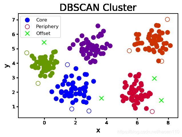
6. DBSCAN(带噪声的基于密度的聚类)算法
-
朋友的朋友也是朋友,从样本空间中任意选择一个样本,以事先给定的半径做圆,凡被该圆圈中的样本都视为与该样本处于相同的聚类,以这些被圈中的样本为圆心继续做圆,重复以上过程,不断扩大被圈中样本的规模,直到再也没有新的样本加入为止,至此即得到一个聚类。于剩余样本中,重复以上过程,直到耗尽样本空间中的所有样本为止。
- 事先给定的半径会影响最后的聚类效果,可以借助轮廓系数选择较优的方案。
- 根据聚类的形成过程,把样本细分为以下三类:
- 外周样本:被其它样本聚集到某个聚类中,但无法再引入新样本的样本。
- 孤立样本:聚类中的样本数低于所设定的下限,则不称其为聚类,反之称其为孤立样本。
- 核心样本:除了外周样本和孤立样本以外的样本。
# dbscan.py
import numpy as np
import sklearn.cluster as sc
import sklearn.metrics as sm
import matplotlib.pyplot as mp
x = []
with open('../data/perf.txt', 'r') as f:
    for line in f.readlines():
        data = [float(substr) for substr in line.split(',')]
        x.append(data)
x = np.array(x)
epsilons, scores, models = np.linspace(0.3, 1.2, 10), [], []
for epsilon in epsilons:
        # DBSCAN聚类器
    model = sc.DBSCAN(eps=epsilon, min_samples=5)
    model.fit(x)
    score = sm.silhouette_score(
        x, model.labels_, sample_size=len(x),
        metric='euclidean')
    scores.append(score)
    models.append(model)
scores = np.array(scores)
best_index = scores.argmax()
best_epsilon = epsilons[best_index]
print(best_epsilon)
best_score = scores[best_index]
print(best_score)
best_model = models[best_index]
pred_y = best_model.fit_predict(x)
core_mask = np.zeros(len(x), dtype=bool)
core_mask[best_model.core_sample_indices_] = True
offset_mask = best_model.labels_ == -1
periphery_mask = ~(core_mask | offset_mask)

mp.figure('DBSCAN Cluster', dpi=120)
mp.title('DBSCAN Cluster', fontsize=20)
mp.xlabel('x', fontsize=14)
mp.ylabel('y', fontsize=14)
mp.tick_params(labelsize=10)
labels = set(pred_y)
cs = mp.get_cmap('brg', len(labels))(range(len(labels)))
mp.scatter(x[core_mask][:, 0], x[core_mask][:, 1],
           c=cs[pred_y[core_mask]], s=80,
           label='Core')
mp.scatter(x[periphery_mask][:, 0], x[periphery_mask][:, 1],
           edgecolor=cs[pred_y[periphery_mask]],
           facecolor='none', s=80, label='Periphery')
mp.scatter(x[offset_mask][:, 0], x[offset_mask][:, 1],
           c=cs[pred_y[offset_mask]], marker='x',
           s=80, label='Offset')
mp.legend()
mp.show()
0.7999999999999999
0.6366395861050828