EM算法实验内容及图片分类任务
EM算法实验内容
一、基本原理
简介
EM算法又称期望最大化算法,是一种迭代算法,是在概率模型中寻找参数极大似然估计的算法,其中概率模型依赖于无法观测的隐含变量。它主要用于从含有隐含变量的数据中计算极大似然估计。是解决存在隐含变量优化问题的有效方法。
简单推导
1. JENSEN不等式
设 f f f是定义域为实数的函数,如果对于所有的实数 x x x, f ” ( x ) ≥ 0 f”(x)≥0 f”(x)≥0,那么 f f f是凸函数。
Jensen不等式表述如下:
E ( f ( X ) ) ≥ f ( E ( X ) ) E(f(X))≥f(E(X)) E(f(X))≥f(E(X))
特别地,如果 f f f是严格凸函数,那么 E ( f ( X ) ) = f ( E ( X ) ) E(f(X))=f(E(X)) E(f(X))=f(E(X))当且仅当,也就是说 X X X是常量。

2. EM算法
(1)完整数据:
-
观测数据:观测到的随机变量 X X X样本
X = ( x 1 , . . . , x n ) X=(x_1,...,x_n) X=(x1,...,xn) -
隐含变量:未观测到的随机变量 Z Z Z的值
Z = ( z 1 , . . . z n ) Z=(z_1,...z_n) Z=(z1,...zn) -
完整数据:包含观测到的随机变量 X X X和隐含变量 Z Z Z的数据: Y = ( X , Z ) Y=(X,Z) Y=(X,Z)
Y = ( ( x 1 , z 1 ) , . . . ( x n , z n ) ) Y=((x_1,z_1),...(x_n,z_n)) Y=((x1,z1),...(xn,zn))
给定的训练样本是 x 1 , x 2 , . . . , x n x_1,x_2,...,x_n x1,x2,...,xn,样例间独立,我们想找到每个样例隐含的类别 z z z,能使得 p ( x , z ) p(x,z) p(x,z)最大。 p ( x , z ) p(x,z) p(x,z)的最大似然估计如下:

EM算法的思想是不断建立 l l l的下界(E-step),然后优化下界(M-step)。
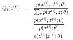
对于每一个样例 i i i,让 Q i Q_i Qi表示该样例隐含变量 z z z的某种分布, Q i Qi Qi满足
Σ z Q i ( z ) = 1 , Q i ( z ) ≥ 0 ΣzQ_i(z)=1,Qi(z)≥0 ΣzQi(z)=1,Qi(z)≥0
得到

这里运用JENSEN不等式,将(3)看成是 θ \theta θ的函数, θ \theta θ又是模型里的参数,上述过程看成是对 l ( θ ) l(\theta) l(θ)求下界的过程,所以(3)是参数 θ \theta θ的对数似然函数的下界。
等式成立的条件为:

c c c为常数,不依赖于 z i z^i zi。对此式子做进一步推导,我们知道 Σ z Q i ( z i ) = 1 ΣzQ_i(z^i)=1 ΣzQi(zi)=1
则
Σ z p ( x i , z i ; θ ) = c Σ_zp(x^i,z^i;θ)=c Σzp(xi,zi;θ)=c
推出下式
3. 算法步骤
- E-step:固定 θ \theta θ后,选择隐含变量 z i z^i zi的概率分布
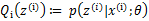
- 在给定 Q i ( z i ) Q_i(z^i) Qi(zi)后,根据求极大似然估计量的过程,去极大化 l ( θ ) l(\theta) l(θ)的下界,得到新的参数 θ \theta θ

二、问题实例
问题
假设有两枚硬币 A、B,以相同的概率随机选择一个硬币,进行如下的抛硬币 实验:共做 5 次实验,每次实验独立的抛十次,结果如图中 a 所示,例如某次实验 产生了 H、T、T、T、H、H、T、H、T、H,H 代表正面朝上。 假设试验数据记录员可能是实习生,业务不一定熟悉,造成如下图的 a 和 b 两种情况:

- a 表示实习生记录了详细的试验数据,我们可以观测到试验数据中每次选择的 是 A 还是 B
- b 表示实习生忘了记录每次试验选择的是 A 还是 B,我们无法观测实验数据中 选择的硬币是哪个
问题求解
1.情况 a
此时清楚的知道抛出的是A还是B,在样本基数很大的情况,可以直接将频率作为概率
θ A = 24 / ( 24 + 6 ) = 0.8 \theta_A=24/(24+6)=0.8 θA=24/(24+6)=0.8
θ B = 9 / ( 9 + 11 ) = 0.45 \theta_B=9/(9+11)=0.45 θB=9/(9+11)=0.45
2. 情况b
已知:硬币正面朝上次数
未知:是A硬币还是B硬币
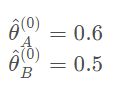
为了得到较为准确的 θ A \theta_A θA和 θ B \theta_B θB,我们使用EM算法,这里假定运算目标的初始值为
E-step
以第一轮抛硬币为例,可以看到5次朝上5次朝下
如果丢的是硬币A,则丢到正面的概率为
P A = C 10 5 ∗ ( θ A ) 5 ∗ ( 1 − θ A ) 10 − 5 P_A=C^5 _{10}*(\theta_A)^5*(1-\theta_A)^{10-5} PA=C105∗(θA)5∗(1−θA)10−5
如果丢的是硬币B,则丢到正面的概率为
P B = C 10 5 ∗ ( θ B ) 5 ∗ ( 1 − θ B ) 10 − 5 P_B=C^5 _{10}*(\theta_B)^5*(1-\theta_B)^{10-5} PB=C105∗(θB)5∗(1−θB)10−5
则在第一轮掷硬币时,该硬币为A的概率为 P A / ( P A + P B ) = 0.45 P_A/(P_A+P_B)=0.45 PA/(PA+PB)=0.45
该硬币为B的概率为
P B / ( p A + p B ) = 0.55 P_B/(p_A+p_B) = 0.55 PB/(pA+pB)=0.55
M-step
此时实际发生正面向上的次数是5,所以这次硬币A正面向上的期望为
5 ∗ 0.45 = 2.2 H 5*0.45=2.2H 5∗0.45=2.2H
同理A反面朝上的概率为
5 ∗ 0.45 = 2.2 T 5*0.45=2.2T 5∗0.45=2.2T
其他轮的运算同理
所有轮运算完,将结果分别对应相加,求出新 θ \theta θ值,即
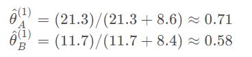
重复E-step和M-step,直至算法收敛到一定精度,结束算法
得到

python实现
已知EM算法是由多次迭代至收敛,所以代码可以分为两个部分。
第一个部分为单次迭代的处理,包括求解二项分布概率质量函数,计算本次抛出硬币分别为A、B的概率,分别计算硬币A、B新的正面朝上的概率。
第二个部分为循环部分,在没有满足设置的收敛条件下,不断进行第一部分的处理,直至达到条件得出结果。
1. 录入数据集
# 硬币投掷结果观测序列
observations = np.array([[1, 0, 0, 0, 1, 1, 0, 1, 0, 1],
                         [1, 1, 1, 1, 0, 1, 1, 1, 1, 1],
                         [1, 0, 1, 1, 1, 1, 1, 0, 1, 1],
                         [1, 0, 1, 0, 0, 0, 1, 1, 0, 0],
                         [0, 1, 1, 1, 0, 1, 1, 1, 0, 1]])
2. 单次迭代em_single
-
这里传入两个数据结构
priors:[theta_A,theta_B]存储了硬币A正面朝上的概率和硬币B正面朝上的概率,在迭代完以后要对其进行更新
observations:[m X n matrix]是一个m*n的矩阵,即前面录入的数据集 -
函数内部数据结构
counts = {"A":{"H":0,"T":0},"B":{"H":0,"T":0}}存储AB硬币统计正反面次数,H正面,T反面
theta_A = priors[0]硬币A 正面朝上的概率
theta_B = priors[1]硬币B正面朝上的概率 -
E-step
- 分别求解硬币A、B的二项分布概率质量函数
#二项分布概率质量函数 contribution_A = stats.binom.pmf(num_heads,len_observation,theta_A) contribution_B = stats.binom.pmf(num_heads,len_observation,theta_B)num_heads为硬币正面朝上的次数
len_observation为这一轮抛硬币的总次数
theta_A/B为达成目标正面朝上的概率
即求抛掷硬币len_observation次(正面概率为theta_A/B),正面朝上num_heads次的概率- 求解抛出硬币分别是A、B的概率
#抛出硬币是A的概率 weight_A = contribution_A / (contribution_A + contribution_B) #抛出硬币是B的概率 weight_B = contribution_B / (contribution_A + contribution_B)- 更新在当前参数下A、B硬币的正反面次数
counts['A']['H'] += weight_A * num_heads counts['A']['T'] += weight_A * num_tails counts['B']['H'] += weight_B * num_heads counts['B']['T'] += weight_B * num_tails -
M-step
分别计算新的A、B正面朝上的概率,并返回
   new_theta_A = counts['A']['H'] / (counts['A']['H'] + counts['A']['T'])
   new_theta_B = counts['B']['H'] / (counts['B']['H'] + counts['B']['T'])
   return [new_theta_A,new_theta_B]
3. 循环多次em
传入参数
"""
EM算法
:param observation: 观测数据
:param prior: 模型初值
:param tol: 迭代结束阈值
:param iterations: 最大迭代次数
:return: 局部最优的模型参数
"""
传入A、B正面朝上的初始概率,在循环中单次迭代(本题中初始概率分别为0.6和0.5)
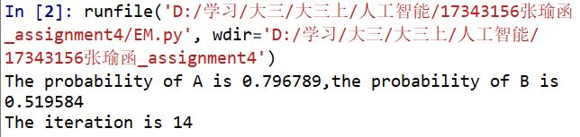
[prob_A,prob_B],iteration = em(observations,[0.6,0.5])
4. 运行结果
图片分类任务
图像分类的任务,就是对于一个给定的图像,预测它属于的那个分类标签(或者给出属于一系列不同标签的可能性)。图像是3维数组,数组元素是取值范围从0到255的整数。数组的尺寸是宽度x高度x3,其中这个3代表的是红、绿和蓝3个颜色通道。
图片分类流程
- 目标:已有固定的分类标签集合,然后对于输入的图像,从分类标签集合中找出一个分类标签,最后把分类标签分配给该输入图像。
- 输入:输入是包含N个图像的集合,每个图像的标签是K种分类标签中的一种。这个集合称为训练集。
- 学习:这一步的任务是使用训练集来学习每个类到底长什么样。一般该步骤叫做训练分类器或者学习一个模型。
- 评价:让分类器来预测它未曾见过的图像的分类标签,并以此来评价分类器的质量。我们会把分类器预测的标签和图像真正的分类标签对比。毫无疑问,分类器预测的分类标签和图像真正的分类标签如果一致,那就是好事,这样的情况越多越好。
图像分类数据集:CIFAR-10
这个数据集包含了60000张32X32的小图像。每张图像都有10种分类标签中的一种。这60000张图像被分为包含50000张图像的训练集和包含10000张图像的测试集。
在运用数据集时要注意的问题:
决不能使用测试集来进行调优,只能使用训练集来调优超参数。测试数据集只使用一次,即在训练完成后评价最终的模型时使用。
调优思路:从训练集中取出一部分数据用来调优,我们称之为验证集(validation set)。
把训练集分成训练集和验证集。使用验证集来对所有超参数调优。最后只在测试集上跑一次并报告结果。
以CIFAR-10为例,我们可以用49000个图像作为训练集,用1000个图像作为验证集。验证集其实就是作为假的测试集来调优。
一、KNN实现
-
Nearest Neighbor图像分类思想
拿测试图片和训练集中每一张图片去比较,然后将它认为最相似的那个训练集图片的标签赋给这张测试图片。 -
比较方法
在本例中,就是比较32x32x3的像素块。最简单的方法就是逐个像素比较,最后将差异值全部加起来。即将两张图片先转化为两个向量 I 1 I_1 I1和 I 2 I_2 I2,然后计算他们的L1距离

这里的求和是针对所有的像素。下面是整个比较流程的图例:
L1方法

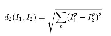
以图片中的一个颜色通道为例来进行说明。两张图片使用L1距离来进行比较。逐个像素求差值,然后将所有差值加起来得到一个数值。如果两张图片一模一样,那么L1距离为0,但是如果两张图片很是不同,那L1值将会非常大。L2方法
计算两个向量间的欧式距离
L1和L2比较
L2比L1更加不能容忍向量的差异。也就是说,相对于1个巨大的差异,L2距离更倾向于接受多个中等程度的差异。L1和L2都是在p-norm常用的特殊形式。 -
KNN分类器
KNN图像分类思想
与其只找最相近的那1个图片的标签,我们找最相似的k个图片的标签,然后让他们针对测试图片进行投票,最后把票数最高的标签作为对测试图片的预测。所以当k=1的时候,k-Nearest Neighbor分类器就是Nearest Neighbor分类器。
k值的选择——交叉验证
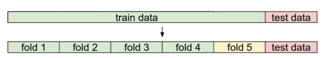
在训练集数量较小的时候(因此验证集的数量更小),我们使用交叉验证的方法。
将训练集平均分成5份,其中4份用来训练,1份用来验证。然后我们循环着取其中4份来训练,其中1份来验证,最后取所有5次验证结果的平均值作为算法验证结果。然后对不同k值的平均表现画线连接。
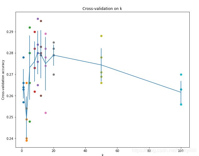
k取准确率峰值的时候,算法表现最好。本例中,当k=10的时算法表现最好。如果我们将训练集分成更多份数,直线一般会更加平滑(噪音更少) -
代码实现
- data_utils载入数据集
def load_CIFAR_batch(filename):
  """ load single batch of cifar """

def load_CIFAR10(ROOT):
  """ load all of cifar """
- testKNN训练和测试
载入数据集的调用
plt.rcParams['figure.figsize'] = (10.0, 8.0) # set default size of plots
plt.rcParams['image.interpolation'] = 'nearest'
plt.rcParams['image.cmap'] = 'gray'

X_train, y_train, X_test, y_test = load_CIFAR10('../datasets')

# As a sanity check, we print out the size of the training and test data.
print('Training data shape: ', X_train.shape)
print('Training labels shape: ', y_train.shape)
print('Test data shape: ', X_test.shape)
print('Test labels shape: ', y_test.shape)
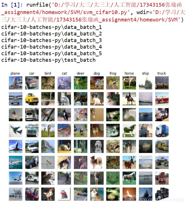
显示数据集的一部分信息
# Visualize some examples from the dataset.
# We show a few examples of training images from each class.
classes = ['plane', 'car', 'bird', 'cat', 'deer', 'dog', 'frog', 'horse', 'ship', 'truck']
num_classes = len(classes)
samples_per_class = 7
for y, cls in enumerate(classes):
    idxs = np.flatnonzero(y_train == y)
    idxs = np.random.choice(idxs, samples_per_class, replace=False)
    for i, idx in enumerate(idxs):
        plt_idx = i * num_classes + y + 1
        plt.subplot(samples_per_class, num_classes, plt_idx)
        plt.imshow(X_train[idx].astype('uint8'))
        plt.axis('off')
        if i == 0:
            plt.title(cls)
plt.show()
截取部分样本数据,以提高本作业的执行效率
num_training = 5000
mask = range(num_training)
X_train = X_train[mask]
y_train = y_train[mask]

num_test = 500
mask = range(num_test)
X_test = X_test[mask]
y_test = y_test[mask]
进行训练
这里对k=1和k=5时训练测试,得到如下结果

测试三种距离计算法的效率
得到如下结果

交叉验证
num_folds = 5
k_choices = [1, 3, 5, 8, 10, 12, 15, 20, 50, 100]

X_train_folds = []
y_train_folds = []
交叉验证实际上是将数据的训练集进行拆分, 分成多个组, 构成多个训练和测试集, 来筛选较好的超参数
数据划分
X_train_folds = np.array_split(X_train, num_folds);
y_train_folds = np.array_split(y_train, num_folds)
找到最佳k值
代码略
- 算法实现
代码用类封装
- train训练分类器。对于KNN算法,此处只需要存储训练数据即可。
- predict基于该分类器,预测测试数据的标签分类。
compute_distances_two_loops,compute_distances_one_loop,compute_distances_no_loops分别是用来实现需要预测的数据集 X 和 原始记录的训练集 self.X_train之间的距离关系, 并通过 predict_labels进行KNN预测
-
compute_distances_two_loops
两层循环计算L2距离

-
compute_distances_one_loop
一层循环计算L2距离,增加axis = 1指定方向 -
compute_distances_no_loops
无循环计算L2距离
数学推导
我们记测试集矩阵为 P P P, 大小为 M × D M×D M×D , 训练集矩阵 为 C C C大小为 N × D N×D N×D
P i P_i Pi是 P P P的第 i i i行, 同理 C j C_j Cj 是 C C C的 第 j j j行:

计算一下 P i P_i Pi 和 C j C_j Cj之间的距离
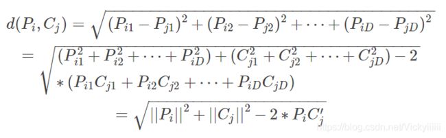
推广得结果矩阵的每行元素为:
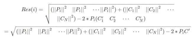
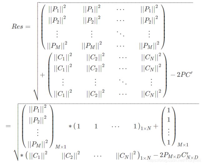
继而, 结果矩阵为:
-
predict_labels
根据计算得到的距离关系, 挑选 K 个数据组成选民, 进行党派选举
KNN运行结果

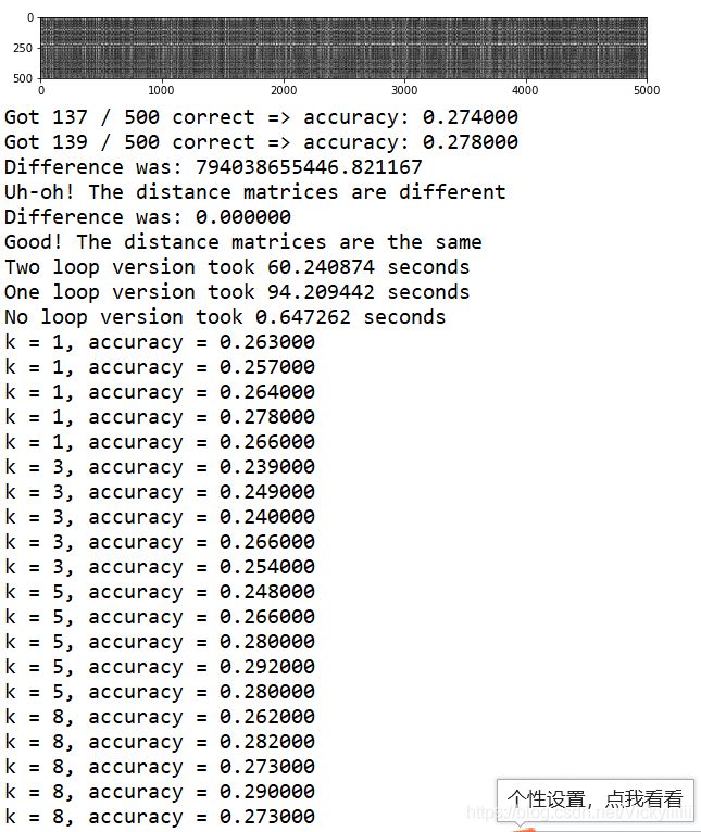

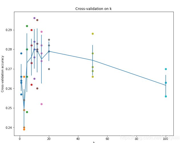
可以看出k=10时最佳,准确率大约为28%
k-Nearest Neighbor分类器的优劣
- 优点
思路清晰,易于理解,实现简单;
算法的训练不需要花时间,因为其训练过程只是将训练集数据存储起来。 - 缺点
测试要花费大量时间计算,因为每个测试图像需要和所有存储的训练图像进行比较。
二、SVM分类
SVM基本思想
简单来说,支持向量机SVM就是在特征空间中找到一条最佳的分类超平面,能够让正、负样本距离该超平面的间隔(margin)最大化。
尽量让所有样本距离分类超平面越远越好。
线性分类与得分函数
在线性分类器算法中,输入为x,输出为y,令权重系数为W,常数项系数为b。我们定义得分函数s为:
s = W x + b s=Wx+b s=Wx+b
这是线性分类器的一般形式,得分函数s所属类别值越大,表示预测该类别的概率越大。
以图像识别为例,共有3个类别「cat,dog,ship」。令输入x的特征维度为4「即包含4个像素值」,W的维度是3x4,b的维度是3x1。在W和b确定后,得到各个类别的得分函数s为:

由上图可知,因为总有3个类别,得分函数s是3x1的向量。其中,cat score=-96.8,dog score=437.9,ship score=61.95。从s的值来说,dog score最高,cat score最低,则预测为狗的概率更大一些。而该图片真实标签是一只猫,显然,从得分函数s上来看,该线性分类器的预测结果是错误的。
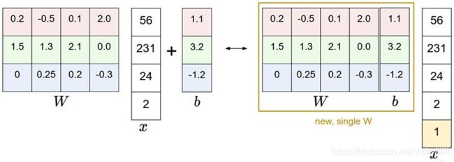
通常为了简化计算,我们直接将W和b整合成一个矩阵,同时将x额外增加一个全为1的维度。这样,得分函数s的表达式得到了简化:

示例图如下:
优化策略与损失函数
正确类别对应的得分函数s应该比其它类别的得分函数s大一个阈值 Δ Δ Δ:
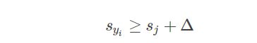
定义SVM的损失函数:
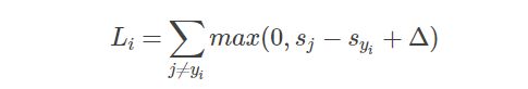

即

其中, y i y_i yi表示正确的类别, j j j表示错误类别。从 L i Li Li的表达式可以看出,只有当 s y i s_{y_i} syi比 s j s_j sj大超过阈值 Δ Δ Δ时, L i L_i Li才为零,否则 L i L_i Li大于零。这种策略类似于距离最大化策略。
这类损失函数的表达式一般称作合页损失函数「Hinge Loss Function」:

显然,只有当 s j − s y i + Δ < 0 s_j−s_{y_i}+Δ<0 sj−syi+Δ<0时,损失函数才为零。
这种合页损失函数的优点是体现了SVM距离最大化的思想;而且,损失函数大于零时,是线性函数,便于梯度下降算法求导。
对于超参数阈值 Δ Δ Δ,一般设置 Δ = 1 Δ=1 Δ=1。因为,权重系数W是可伸缩的,直接影响着得分函数s的大小。所以说, Δ = 1 Δ=1 Δ=1或 Δ = 10 Δ=10 Δ=10,实际上没有差别,对W的伸缩完全可以抵消掉 Δ Δ Δ 的数值影响。因此,通常把 Δ Δ Δ 设置为1即可。此时的损失函数为:

SVM中,为了防止模型过拟合,可以使用正则化「Regularization」方法。例如使用L2正则化:

引入正则化项之后的损失函数为:

其中,N是训练样本个数, λ λ λ是正则化参数,可调。一般来说, λ λ λ 越大,对权重W的惩罚越大; λ λ λ 越小,对权重W的惩罚越小。 λ λ λ 实际上是权衡损失函数第一项和第二项之间的关系:
- λ λ λ 越大,对W的惩罚更大,牺牲正负样本之间的间隔,可能造成欠拟合「underfit」;
- λ λ λ 越小,得到的正负样本间隔更大,但是W数值会变大,可能造成过拟合「overfit」。
实际应用中,可通过交叉验证,选择合适的正则化参数 λ λ λ。
程序实现
用SVM类封装
- 计算loss和gredients
def svm_cost_function(self, X, y, reg, delta):
        """ cal loss

        :param X: A numpy array of shape (N, D)
        :param y: A numpy array of shape (N, )
        :param reg: regularization strength
        :param delta: margin
        :return: loss, gred
        """
        num_train = X.shape[0]

        scores = X.dot(self.W.T)  # N * C
        correct_class_scores = scores[range(num_train), y]
        margins = scores - correct_class_scores[:, np.newaxis] + delta
        margins = np.maximum(0, margins)
        # do not ignore it, because 'y - y + delta' > 0, we should reset it to zeros
        margins[range(num_train), y] = 0

        loss = np.sum(margins) / num_train + 0.5 * reg * np.sum(self.W * self.W)

        # cal gred [for every example, when margin > 0, correct lable's W should -X, and wrong lable's W should +X]
        ground_true = np.zeros(margins.shape)  # N * C
        ground_true[margins > 0] = 1
        sum_margins = np.sum(ground_true, axis=1)
        ground_true[range(num_train), y] -= sum_margins

        gred = ground_true.T.dot(X) / num_train + reg * self.W

        return loss, gred
- 实现神经网络的训练,用到上面的svm_cost_function函数,采用Stochastic Gradient Descent,即每次迭代不用全部的训练集作为训练而是抽取部分样本,进行多次迭代
def train(self, X, y, reg, delta, learning_rate, batch_num, num_iter, output):
        """ train SVM

        :param X: A numpy array of shape (N, D)
        :param y: A numpy array of shape (N, )
        :param reg: A numpy array of shape (N, )
        :param delta: margin
        :param learning_rate: gradient descent rate
        :param batch_num: training examples to use at each step in Mini-batch gradient descent
        :param num_iter: number of steps to take when optimizing
        :return: loss_history
        """
        num_train = X.shape[0]
        num_dim = X.shape[1]
        num_classes = np.max(y) + 1  # y takes values 0...K-1

        if self.W is None:
            # lazily initialize W
            self.W = 0.001 * np.random.randn(num_classes, num_dim)

        # train
        loss_history = []
        for i in range(num_iter):
            # Mini-batch
            sample_index = np.random.choice(num_train, batch_num, replace=False)
            X_batch = X[sample_index, :]
            y_batch = y[sample_index]

            loss, gred = self.svm_cost_function(X_batch, y_batch, reg, delta)
            loss_history.append(loss)
            self.W -= learning_rate * gred

            if output and  i % 100 == 0:
                    print('Iteration %d / %d: loss %f' % (i, num_iter, loss))

        return loss_history
返回loss_history
- 使用这个网络模型的训练权重来预测数据
def predict(self, X):
        """ predict

        :param X: A numpy array of shape (N, D)
        :return: y_pred (A numpy array of shape (N, ))
        """
        ...
        return y_pred
- 运行过程
对数据集的处理这里不做赘述
main函数调用以下函数来完成测试
if __name__ == '__main__':
    # 对数据进行预处理,得到训练集,测试集,验证集
    X_train, y_train, X_test, y_test, X_val, y_val = pre_dataset()
    # 通过验证集自动化确定参数 learning_rate和reg
    best_parameter = auto_get_parameter(X_train, y_train, X_val, y_val)
    # 通过参数和训练集构建SVM模型
    svm = get_svm_model(best_parameter, X_train, y_train)
    # 用测试集预测准确率
    y_pred = svm.predict(X_test)
    print('Accuracy achieved during cross-validation: %f' % (np.mean(y_pred == y_test)))
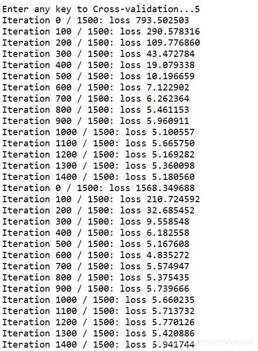
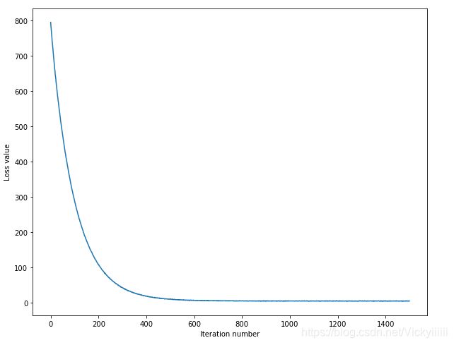
运行结果
交叉验证,可看到loss_history,寻找最适合的超参数
…

…
输入一个超参数,可预测准确率

可以看到与KNN相比,准确率有了较大的提升
三、两层神经网络
线性模型具有局限性
两层神经网络基本步骤
1、反向求导
2、数据预处理
一般采用减均值,若特征间数据的范围差距很大,则考虑除以均方差进行归一化。一般不需要PCA降维和白化操作
切记先切分数据集、验证集、测试集,之后再进行预处理
3、初始化
权重初始化
w = np.random.randn(n) * np.sqrt(2/n)
#后续再卷积神经网络中测试`
偏置初始化b = 0
多层网络间正则化程度一般取相同,可采用L2正则化和随机失活
4、检查解析梯度
使用少量数据点加快检查速度,检查时先将正则化为0,避免正则化过大掩盖了数据损失部分,之后可以加上正则化进行检查,检查时记得关闭随机失活等不确定性。
5、合理性检查
可进行小参数初始化,检查期望值与实际值的差距;提高正则化强度,观察损失函数变化;对小数据集上对数据进行过拟合,看是否可以达到0损失函数值,如果不行,则模型算法有误。
6、观察学习过程中的重要数值的变化
损失函数值(每epoch周期的变化情况),验证集与测试集的正确率(不应差距过大,也不可以完全贴合),权重更新比例(dw/w)一般为1e-3,否则修改步长。
7、采用SGD
8、使用交叉验证来获取最佳超参数,参数范围建议采用随机搜索(比较宽的范围训练后训练比较窄的范围)
实现
搭建神经网络简化结构如图,对Cifar-10数据集进行分类

前向传播
假设有m个输入样例,并且每个输入样例有n个输入特征,则 X X X为n行m列矩阵。对于每一个隐藏单元,都对应于一个列向量w和b,因此 W 1 W1 W1为n行4列的矩阵, B 1 B1 B1为列向量(长为4)。
则 Z 1 = n p . d o t ( W 1. T , X ) + B 1 Z1 = np.dot(W1.T , X) + B1 Z1=np.dot(W1.T,X)+B1为4行m列的矩阵, Y 1 h a t = s i g m o d ( Z 1 ) Y1_hat=sigmod(Z1) Y1hat=sigmod(Z1)表示隐藏单元的输入值。接下来就变成以 Y 1 h a t Y1_hat Y1hat作为输入的单个神经单元。 Z 2 = n p . d o t ( w 2. T , Y 1 h a t ) + b 2 Z2 = np.dot(w2.T, Y1_hat) + b2 Z2=np.dot(w2.T,Y1hat)+b2, y 2 h a t = s i g m o d ( z 2 ) y2_hat = sigmod(z2) y2hat=sigmod(z2)即为最终输出值
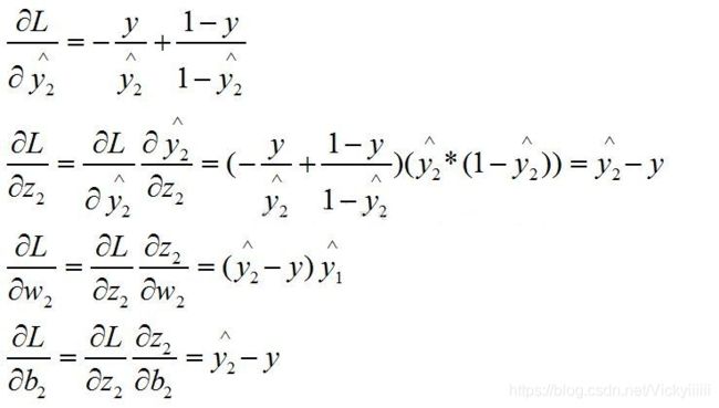
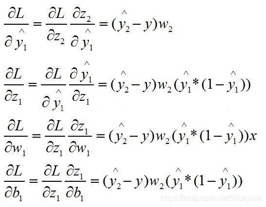
反向传播
根据基于神经网络的二分类问题中定义的损失函数,这里给出单个样例的各个参数的偏导公式推导。
第二层反向过程:
第一层反向过程:
- 参数初始化
def __init__(self, input_size, hidden_size, num_classes, std=1e-4):
        """
        Weights are initialized to small random values and biases are initialized to zero.
        """
        self.parameters = {}
        self.parameters['W1'] = std * np.random.randn(hidden_size, input_size)
        self.parameters['b1'] = np.zeros(hidden_size)
        self.parameters['W2'] = std * np.random.randn(num_classes, hidden_size)
        self.parameters['b2'] = np.zeros(num_classes)
- 计算loss以及gradient
def loss(self, X, y, reg):
        """
        计算两层全连接神经网络的loss和gradients
        输入:
        X: N * D
        y: N * 1
        reg : 正则化强度

        返回:
        如果y是None,返回维数为(N,C)的分数矩阵
        如果y 不是None ,则返回一个元组:
        - loss : float 类型,数据损失和正则化损失
        - grads : 一个字典类型,存储W1,W2,b1,b2的梯度
        """
         # Unpack variables from the params dictionary
        ...

        # Compute the forward pass
        Relu = lambda x: np.maximum(0, x)
        z1 = X.dot(W1.T) + b1  # N * H
        a1 = Relu(z1)
        z2 = a1.dot(W2.T) + b2  # N * C
        scores = z2

         # If the targets are not given then jump out, we're done
        ...

        # Compute the loss
        exp_scores = np.exp(scores - np.max(scores, axis=1, keepdims=True))
        pro_scores = exp_scores / np.sum(exp_scores, axis=1, keepdims=True)
        ground_true = np.zeros(scores.shape)
        ground_true[range(num_examples), y] = 1
        loss = -np.sum(ground_true * np.log(pro_scores)) / num_examples + 0.5 * reg * (np.sum(W1 * W1) + np.sum(W2 * W2))

        # Backward pass: compute gradients
        grads = {}
        # Compute the gradient of z2 (scores)
        dz2 = -(ground_true - pro_scores) / num_examples  # N * C
        # Backprop into W2, b2 and a1
        dW2 = dz2.T.dot(a1)  # C * H
        db2 = np.sum(dz2, axis=0)  # 1 * C
        da1 = dz2.dot(W2)  # N * H
        # Backprop into z1
        ...
        # Backprop into W1, b1
        ...

        # add the regularization
        ...

        return loss, grads
- 实现神经网络的训练
def train(self, X, y, X_val, y_val, reg, learning_rate,
                learning_rate_decay, iterations_per_lr_annealing,
                num_epoches, batch_size, verbose):


        num_examples = X.shape[0]
        # Use SGD to optimize the parameters in self.model
        loss_history = []
        train_acc_history = []
        val_acc_history = []
        iterations_per_epoch = max(num_examples / batch_size, 1)
        num_iters = int(num_epoches * iterations_per_epoch)

        for i in range(num_iters):
            # mini batch
            sample_index = np.random.choice(num_examples, batch_size, replace=True)
            X_batch = X[sample_index, :]
            y_batch = y[sample_index]

            # Compute loss and gradients using the current minibatch
            loss, grads = self.loss(X_batch, y_batch, reg)
            loss_history.append(loss)

             # Use the gradients in the grads dictionary to update
            self.parameters['W1'] -= learning_rate * grads['W1']
            self.parameters['b1'] -= learning_rate * grads['b1']
            self.parameters['W2'] -= learning_rate * grads['W2']
            self.parameters['b2'] -= learning_rate * grads['b2']

            if verbose and i % 100 == 0:
                print('iteration %d / %d: loss %f' % (i, num_iters, loss))

             # Every epoch, check train and val accuracy and decay learning rate.
            if i % iterations_per_epoch == 0:
                train_acc_history.append(np.mean(self.predict(X_batch) == y_batch))
                val_acc_history.append(np.mean(self.predict(X_val) == y_val))

            if i % iterations_per_lr_annealing == 0:
                # Decay learning rate
                learning_rate *= learning_rate_decay

        return {
            'loss_history': loss_history,
            'train_acc_history': train_acc_history,
            'val_acc_history': val_acc_history
        }
- 神经网络的预测
def predict(self, X):
         """
        使用这个网络模型的训练权重来预测数据
        输入:
        - X : (N,D)
        返回:
        - y_pred : (N, )
        """
        # Compute the forward pass
        Relu = lambda x: np.maximum(0, x)
        z1 = X.dot(self.parameters['W1'].T) + self.parameters['b1']
        a1 = Relu(z1)
        z2 = a1.dot(self.parameters['W2'].T) + self.parameters['b2']
        score = z2

        y_pred = np.argmax(score, axis=1)
        return y_pred
- 加载Cifar-10数据集进行图片的分类
if __name__ == '__main__':
    X_train, y_train, X_test, y_test, X_val, y_val = pre_dataset('cifar-10-batches-py')
    best_net = auto_get_parameters(X_train, y_train, X_val, y_val)
    test_acc = np.mean(best_net.predict(X_test) == y_test)
    print('Test accuracy: {}'.format(test_acc))
运行结果

交叉验证

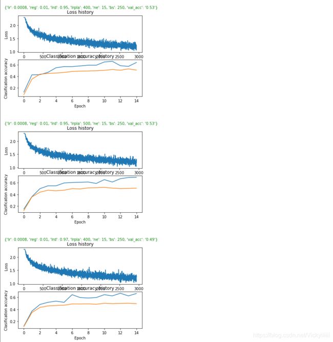
…

可以看到准确率为50%左右
张瑜函 中山大学人工智能作业