Introduction to Graph Neural Network (GNN) 图神经网络入门详解

往期文章链接目录

Note

This is the first post of the Graph Neural Networks (GNNs) series.

Background and Intuition

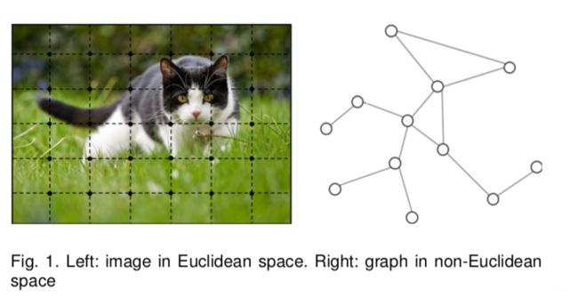
There is an increasing number of applications where data are generated from non-Euclidean domains and are represented as graphs with complex relationships and interdependency between objects. For examples, in e-commence, a graph-based learning system can exploit the interactions between users and products to make highly accurate recommendations. In chemistry, molecules are modeled as graphs.

Another example is the image data. We can represent an image as a regular grid in the Euclidean space. A convolutional neural network (CNN) is able to exploit the shift-invariance, local connectivity, and compositionality of image data. As a result, CNNs can extract local meaningful features that are shared with the entire data sets for various image analysis.

As graphs can be irregular, a graph may have a variable size of unordered nodes, and nodes from a graph may have a different number of neighbors, resulting in some important operations (e.g., convolutions) being easy to compute in the image domain, but difficult to apply to the graph domain.

Furthermore, a core assumption of existing machine learning algorithms is that instances are independent of each other. This assumption no longer holds for graph data because each node is related to others by links of various types, such as citations, friendships, and interactions.

The complexity of graph data has imposed significant challenges on existing machine learning algorithms, and nowadays many studies on extending deep learning approaches for graph data have emerged.

Intro to Graph Neural Networks

Graph neural networks (GNNs) are categorized into four groups:

• Recurrent graph neural networks (RecGNNs)
• Convolutional graph neural networks (ConvGNNs)
• Graph autoencoders (GAEs)
• Spatial-temporal graph neural networks (STGNNs).

These early studies fall into the category of recurrent graph neural networks (RecGNNs). They learn a target node’s representation by propagating neighbor information in an iterative manner until a stable fixed point is reached. This process is computationally expensive, and recently there have been increasing efforts to overcome these challenges.

Encouraged by the success of CNNs in the computer vision domain, a large number of methods that re-define the notion of convolution for graph data are developed in parallel. These approaches are under the umbrella of convolutional graph neural networks (ConvGNNs). ConvGNNs are divided into two main streams, the spectral-based approaches and the spatial-based approaches.

GNNs Framework

With the graph structure and node content information as inputs, the outputs of GNNs can focus on different graph analytics tasks with one of the following mechanisms:

• Node-level outputs relate to node regression and node classification tasks. RecGNNs and ConvGNNs can extract high-level node representations by information propagation/graph convolution. With a multi-perceptron or a softmax layer as the output layer, GNNs are able to perform node-level tasks in an end-to-end manner.

• Edge-level outputs relate to the edge classification and link prediction tasks. With two nodes’ hidden representations from GNNs as inputs, a similarity function or a neural network can be utilized to predict the label/connection strength of an edge.

• Graph-level outputs relate to the graph classification task. To obtain a compact representation on the graph level, GNNs are often combined with pooling and readout operations.

Definition

A graph is represented as $G=(V,E)$ where

• $V$ is the set of nodes/ vertices, $v_i\in$ $V$ denotes a node in $V$;
• $E$ is the set of edges;
• The neighborhood of a node $v$ is defined as $N(v)=\{u\in V\mid (v,u)\in E\}$.

We are going to use the following notations in the post:

• $X\in {\mathbf{R}}^{n\times d}$: The feature matrix of the graph, which is a concatenation of all node representations of the graph. $n$ is the number of nodes and $d$ is the dimension of a node feature vector.
• ${\mathbf{x}}_v$: feature at node $v$.
• ${\mathbf{x}}_{(v,u)}$: feature at the edge between node the $v$ and the node $u$.
• $\mathbf{H}\in {\mathbf{R}}^{n\times b}$: The node hidden feature matrix, where $b$ is the dimension of a hidden node feature vector.
• ${\mathbf{h}}_v\in {\mathbf{R}}^b$: hidden state embedding for the node $v$.

Recurrent graph neural networks (RecGNNs)

Introduction to RecGNNs

Recurrent graph neural networks (RecGNNs) mostly are pioneer works of graph neural networks which are based on the fixed point theorem. The primary goal of RecGNNs is to learn an embedding for each node (node representation). More specifically, given a graph G, each node $x_v$ and edge $x_{(v,u)}$ connecting two nodes $x_v,x_u$ has its own feature, and the goal is to learn these features.

RecGNNs aim to learn these node representations with recurrent neural architectures. They apply the same set of parameters recurrently over nodes in a graph to extract high-level node representations. They assume a node in a graph constantly exchanges information/ message with its neighbors until a stable equilibrium is reached. RecGNNs are conceptually important and inspired later research on convolutional graph neural networks.

Based on an information diffusion mechanism, RecGNNs updates nodes’ states by exchanging neighborhood information recurrently until a stable equilibrium is reached. A node’s hidden state is recurrently updated by

$${\mathbf{h}}_v^{(t)}=\sum _{u\in N(v)}f\left({\mathbf{x}}_v,{\mathbf{x}}_{(v,u)},{\mathbf{x}}_u,{\mathbf{h}}_u^{(t-1)}\right)\text{\hspace{1em}(1)}$$

where

• $f(\cdot )$ is a parametric function (also called local transaction function) which could be approximated by a neural network
• ${\mathbf{h}}_v^{(0)}$ is initialized randomly
• The sum operation enables RecGNNs to be applicable to all nodes, even if the number of neighbors differs.

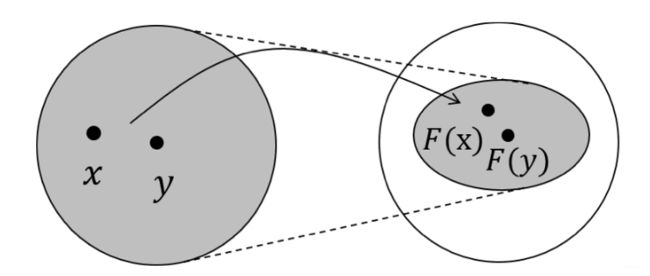
To ensure convergence, the recurrent function $f(\cdot )$ must be a contraction mapping, which shrinks the distance between two points after projecting them into a latent space. Notice that when a convergence criterion is satisfied, the last step node hidden states are the final node embeddings/ representations. Then a local output function $g$ is added for the following downstream tasks. For example, we use

$${\mathbf{o}}_v=g\left({\mathbf{h}}_v,{\mathbf{x}}_v\right)\text{\hspace{1em}(2)}$$

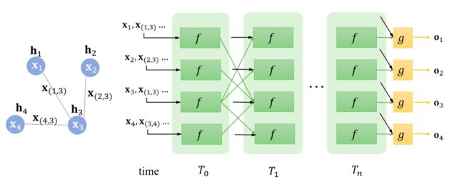
to describe how the output is produced. The pipeline could be visualized as the following figure:

Note how the connections (green lines) match the sample graph on the left. From (1), the input of the first cell is ${\mathbf{x}}_1,{\mathbf{x}}_{(1,3)},{\mathbf{x}}_3,{\mathbf{h}}_3$. After convergence, a local output function $g$ is added to produce output.

Banach’s Fixed Point Theorem

Let $F$ be a function obtained by stacking several $f$ together (aka global transition function). The fixed point theorem suggests that if $F$ is a contraction mapping, then $H$ will always converge to a fixed point regardless of what $H^0$ is.

In other words, after contraction mapping $F$, the image after mapping must be smaller than the original space. Imagine that this compression process continues, eventually all points in the original space will be mapped to one point.

• contraction mapping: a function $F$ from $M$ to itself, with the property that there is some nonnegative real number $0\le k<1$ such that for all $x$ and $y$ in $M$,

$$d(F(x),F(y))\le kd(x,y)\text{\hspace{1em}(3)}$$

Let F be a neural netwrok, to make sure F is a contraction mapping, a penalty term has to be imposed on the Jacobian matrix of parameters. To illustrate the point, let x, y be two vectors in an one dimensional space, then from the definition of the contraction mapping, we have

$$\begin{array}{c}\Vert F(x)-F(y)\Vert \le c\Vert x-y\Vert ,0\le c<1\\ \frac{\Vert F(x)-F(y)\Vert }{\Vert x-y\Vert }\le c\\ \frac{\Vert F(x)-F(x-\Delta x)\Vert }{\Vert \Delta x\Vert }\le c\\ \Vert F^{\prime }(x)\Vert =\Vert \frac{\partial F(x)}{\partial x}\Vert \le c\end{array}$$

Notice that to be a contraction mapping, the gradient has to be less than $1$. We use Lagrange Multiplier to convert this constrained problem to an un-constrained problem and the training objective can be written as

$$J=\mathrm{Loss}+\lambda \cdot \max \left(\frac{\Vert \partial F\Vert }{\Vert \partial \mathbf{h}\Vert }-c,0\right),c\in (0,1)\text{\hspace{1em}(4)}$$

with hyper-parameter $\lambda$. The penalty term is a hinge loss.

After setting up labels for nodes’ outputs, we could then update parameters by calculating the gradient of the back-propagation based on the loss from the forward-propagation.

RecGNNs v.s. RNNs

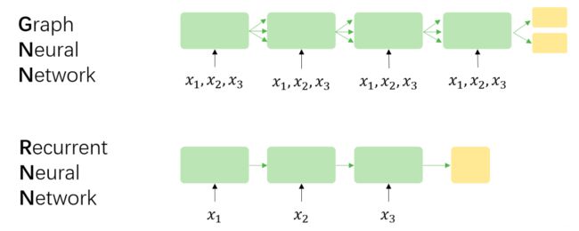
For simplicity, assuming that there are three nodes ${\mathbf{x}}_1,{\mathbf{x}}_2,{\mathbf{x}}_3$ in GNN. Correspondingly, there is a sequence $({\mathbf{x}}_1,{\mathbf{x}}_2,{\mathbf{x}}_3)$ in RNN. The followings are the differences:

• RecGNNs are based on the fixed point theorem, which means that the length of RecGNNs unfolded along time is dynamic and determined according to the convergence conditions, while the length of RNNs unfolded along time is equal to the length of the sequence itself.

• The input of each time step of RecGNNs is features of all nodes and edges, and the input of each time step of RNNs is the corresponding input at that moment. At the same time, the information flow between time steps is not the same, the former is determined by the edge, and the latter is determined by the order of the input sequence.

• The goal of RecGNNs is to obtain a stable hidden state for each node, so it has outputs only after the hidden state converges; while RNN can output at each time step.

• RecGNNs uses Almeida-Pineda (AP) algorithm to optimize back-propagation, while RNNs uses Back Propogation Through Time (BPTT). The former has requirements for convergence, while the latter does not.

Limitation of RecGNNs

• There is limited influence of edges on the hidden state of nodes, and RecGNNs do not have learnable parameters for edges, which means that certain features of edges cannot be learned by the model.

• Fixed point theorem will lead to too much information sharing between the hidden states of nodes, resulting in the over-smoothing problem, and node representations become less informative (all look similiar). Here is an illustration of over-smoothing problem:

Note: The purpose of using the fix point theorem is to make sure RecGNNs is stable. However, if the model is too deep, all hidden states of nodes will be similar (over-smoothing as stated above).

Gated Graph Neural Networks (GGNNs)

Introduction to GGNNs

Gated Graph Neural Network (GGNN) employs a gated recurrent unit (GRU) as a recurrent function, reducing the recurrence to a fixed number of steps. The advantage is that it no longer needs to constrain parameters to ensure convergence. A node hidden state is updated by its previous hidden states and its neighboring hidden states, defined as

$${\mathbf{h}}_v^{(t)}=GRU\left({\mathbf{h}}_v^{(t-1)},\sum _{u\in N(v)}{\mathbf{W}}_{edge}{\mathbf{h}}_u^{(t-1)}\right)$$

where ${\mathbf{h}}_v^{(0)}={\mathbf{x}}_v$ and ${\mathbf{W}}_{edge}$ consists of learnable parameters for edges. Notice that different from RecGNNs, node features ${\mathbf{x}}_v$ do not appear in the formula of GGNN, but instead used as initialization of hidden states of nodes.

GGNNs v.s. RecRNNs

The major difference between GGNNs and RecRNNs is that GGNNs are longer based on the fixed point theorem, which means that the convergence is no longer required.

Other than that, GGNNs use the BPTT algorithm to learn the model parameters. This can be problematic for large graphs, as GGNNs need to run the recurrent function multiple times over all nodes, requiring the intermediate states of all nodes to be stored in memory.

---

Reference:

• https://en.wikipedia.org/wiki/Contraction_mapping
• Big thanks to this blog: From graph to graph convolution (1): https://www.cnblogs.com/SivilTaram/p/graph_neural_network_1.html
• https://en.wikipedia.org/wiki/File:Graph_Laplacian_Diffusion_Example.gif

Paper:

• A Comprehensive Survey on Graph Neural Networks: https://arxiv.org/pdf/1901.00596.pdf
• The graph neural network model: https://persagen.com/files/misc/scarselli2009graph.pdf
• Gated Graph Sequence Neural Networks: https://arxiv.org/pdf/1511.05493.pdf

往期文章链接目录