计算机视觉(九)——KNN算法和稠密SIFT实现手势识别
博文主要内容
- KNN(K近邻分类法)实现数据分类
- DSIFT(稠密SIFT)不同图像识别
- DSIFT(稠密SIFT)实现手势识别
KNN(K近邻分类法)原理介绍
KNN算法又称K近邻分类法,是一种使用最多的分类算法之一。它通过将需要分类的对象数据,与训练完成的已知类别标记的所有对象进行对比,并由k近邻对指派到哪个类别进行投票。通俗的讲,在已知分好类别的数据中,你投入一个新的数据,计算这个数据周边一定范围之内,计算不同类别数据的数量,根据数量进行投票,最终确定好投入数据的类别。
KNN(K近邻分类法)实现数据分类实验代码
1.生成训练数据和测试数据
# -*- coding: utf-8 -*-
from numpy.random import randn
import pickle
from pylab import *

# create sample data of 2D points
n = 200
# two normal distributions
class_1 = 0.5 * randn(n,2)
class_2 = 4.0 * randn(n,2) + array([8,8])
labels = hstack((ones(n),-ones(n)))

# save with Pickle
#with open('points_normal_test.pkl', 'w') as f:
with open('points_normal.pkl', 'w') as f:
    pickle.dump(class_1,f)
    pickle.dump(class_2,f)
    pickle.dump(labels,f)
# normal distribution and ring around it
print "save OK!"
class_1 = 0.4 * randn(n,2)
r = 0.8 * randn(n,1) + 7
angle = 2*pi * randn(n,1)
class_2 = hstack((r*cos(angle),r*sin(angle)))
labels = hstack((ones(n),-ones(n)))
# save with Pickle
#with open('points_ring_test.pkl', 'w') as f:
with open('points_ring.pkl', 'w') as f:
    pickle.dump(class_1,f)
    pickle.dump(class_2,f)
    pickle.dump(labels,f)

print "save OK!"
需要注意的是,代码中有#with open('points_normal_test.pkl', 'w') as f:和#with open('points_ring_test.pkl', 'w') as f:这两句被注释之后的代码,这是用来生成测试数据的,使用时先运行一遍,将这两句解除注释,并注释下一行类似的代码,就会生成

如果所示的四个文件。
关于数据集的选取,这里通过随机数randn来控制生成需要的数据,class_1 class_2是数据的分类点。
class_1 = 0.5 * randn(n,2)
class_2 = 4.0 * randn(n,2) + array([8,8])
class_1表示为标准差为0.5的标准正态分布的随机二维矩阵。class_2是均值在(8,8),标准差为4的正态分布的随机二维矩阵
同理在points_ring中class_2是通过生成r和angle计算其在X轴与Y的投影作为数据。
最后,按照所说运行之后会出现两个save OK!
2.对数据进行分类
# -*- coding: utf-8 -*-
import pickle
from pylab import *
from PCV.classifiers import knn
from PCV.tools import imtools

pklist=['points_normal.pkl','points_ring.pkl']

figure()

# load 2D points using Pickle
for i, pklfile in enumerate(pklist):
    with open(pklfile, 'r') as f:
        class_1 = pickle.load(f)
        class_2 = pickle.load(f)
        labels = pickle.load(f)

    model = knn.KnnClassifier(labels, vstack((class_1, class_2)))

        # load test data using Pickle
    with open(pklfile[:-4]+'_test.pkl', 'r') as f:
        class_1 = pickle.load(f)
        class_2 = pickle.load(f)
        labels = pickle.load(f)

    print pklfile

    # test on the first point
    print model.classify(class_1[0])

    #define function for plotting
    def classify(x,y,model=model):
        return array([model.classify([xx,yy]) for (xx,yy) in zip(x,y)])

    # lot the classification boundary
    subplot(1,2,i+1)
    imtools.plot_2D_boundary([-6,6,-6,6],[class_1,class_2],classify,[1,-1])
    titlename=pklfile[:-4]
    title(titlename)
show()
数据分类先通过points_normal和points_ring来生成模型,通过这个模型来测试对测试数据的分类。
测试的数据分类如下。分别是普通的两类分类和圆环类型的分类。
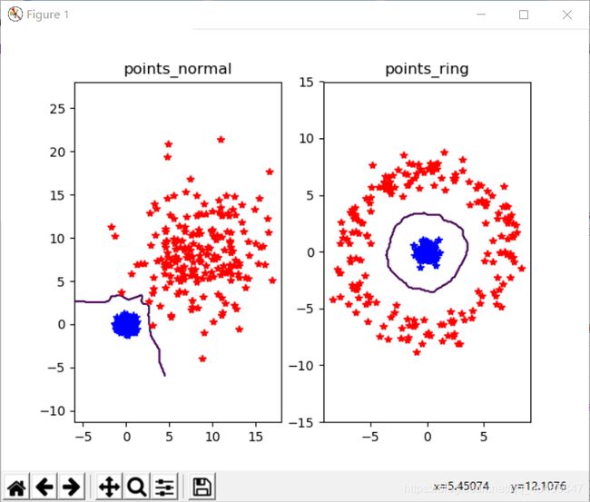
因为randn是一个标准正态分布的随即数据,所以在第一张图的因为class_2给的标准差过大,就出现了数据占据大块面积的情况。
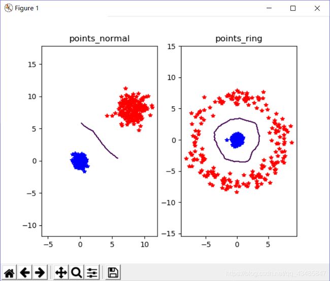
这是我把标准差改成1.1之后的数据分类,代码class_2 = 1.1 * randn(n,2) + array([8,8])。相比之前的,缩小标准差使得数据收敛,于是分类就变得比较明显了。
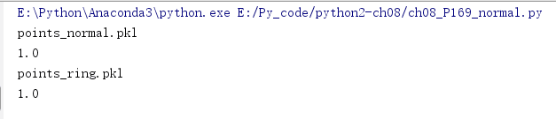
这是运行代码之后的输出。points_normal和points_ring分别表示着程序进行什么数据的分类过程。
DSIFT(稠密SIFT)原理介绍
DSIFT(稠密SIFT)算法是在SIFT算法上进行改进的算法。DSIFT有三个特点:
- 在DSIFT算法下,仍然保留着SIFT对尺度缩放以及亮度变化的不变性,在视角变换、仿射变换以及噪声也保留一定的稳定性。
- 在时间上,DSIFT相比SIFT有所减少。
- 相比SIFT,DSIFT的特征分布更加平均。
简单来讲DSIFT通过将图像每一块划分,在进行DSIFT,具体划分效果在实验中可以看到。
DSIFT(稠密SIFT)不同图像识别和手势识别
1.DSIFT(稠密SIFT)不同图像识别实现
# -*- coding: utf-8 -*-
from PCV.localdescriptors import sift, dsift
from pylab import  *
from PIL import Image

dsift.process_image_dsift('E:/Py_code/photo/z/17.jpg','17.dsift',90,40,True)
l,d = sift.read_features_from_file('17.dsift')
im = array(Image.open('E:/Py_code/photo/z/17.jpg'))
sift.plot_features(im,l,True)
title('dense SIFT')
show()
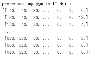
这就是对图像进行DSIFT特征提取,图像中的小圆圈就是DSIFT算法将图像每一处进行分割的标记结果。以及输出框的输出。

2.DSIFT(稠密SIFT)实现手势识别
# -*- coding: utf-8 -*-
import os
from PCV.localdescriptors import sift, dsift
from pylab import  *
from PIL import Image

imlist=['E:/Py_code/photo/ch08/train/1_01.jpg','E:/Py_code/photo/ch08/train/C_01.jpg',
        'E:/Py_code/photo/ch08/train/V_01.jpg','E:/Py_code/photo/ch08/train/5_01.jpg',]

figure()
for i, im in enumerate(imlist):
    print im
    dsift.process_image_dsift(im,im[:-3]+'dsift',90,40,True)
    l,d = sift.read_features_from_file(im[:-3]+'dsift')
    dirpath, filename=os.path.split(im)
    im = array(Image.open(im))
    #显示手势含义title
    titlename=filename[:-4]
    subplot(2,2,i+1)
    sift.plot_features(im,l,True)
    title(titlename)
show()
因为在自己建立手势姿势时候,就只使用4种手势,所以输出如下:

需要注意的是,在titlename=filename[:-4]这句中,想要在输出的图像中显示手势名称,需要将后面的 -4 做修改,改成你图像的名称的长度就是出现图中的结果。
3.DSIFT(稠密SIFT)实现多张手势识别
# -*- coding: utf-8 -*-
from PCV.localdescriptors import dsift
import os
from PCV.localdescriptors import sift
from pylab import *
from PCV.classifiers import knn

def get_imagelist(path):
    """    Returns a list of filenames for
        all jpg images in a directory. """

    return [os.path.join(path,f) for f in os.listdir(path) if f.endswith('.jpg')]

def read_gesture_features_labels(path):
    # create list of all files ending in .dsift
    featlist = [os.path.join(path,f) for f in os.listdir(path) if f.endswith('.dsift')]
    # read the features
    features = []
    for featfile in featlist:
        l,d = sift.read_features_from_file(featfile)
        features.append(d.flatten())
    features = array(features)
    # create labels
    labels = [featfile.split('/')[-1][0] for featfile in featlist]
    return features,array(labels)

def print_confusion(res,labels,classnames):
    n = len(classnames)
    # confusion matrix
    class_ind = dict([(classnames[i],i) for i in range(n)])
    confuse = zeros((n,n))
    for i in range(len(test_labels)):
        confuse[class_ind[res[i]],class_ind[test_labels[i]]] += 1
    print 'Confusion matrix for'
    print classnames
    print confuse

filelist_train = get_imagelist('E:/Py_code/photo/ch08/train')
filelist_test = get_imagelist('E:/Py_code/photo/ch08/test')
imlist=filelist_train+filelist_test

# process images at fixed size (50,50)
for filename in imlist:
    featfile = filename[:-3]+'dsift'
    dsift.process_image_dsift(filename,featfile,10,5,resize=(50,50))

features,labels = read_gesture_features_labels('E:/Py_code/photo/ch08/train/')
test_features,test_labels = read_gesture_features_labels('E:/Py_code/photo/ch08/test/')
classnames = unique(labels)

# test kNN
k = 1
knn_classifier = knn.KnnClassifier(labels,features)
res = array([knn_classifier.classify(test_features[i],k) for i in
range(len(test_labels))])
# accuracy
acc = sum(1.0*(res==test_labels)) / len(test_labels)
print 'Accuracy:', acc

print_confusion(res,test_labels,classnames)
这段代码是通过将图像分成两个文件夹,train和test两个文件夹来实现训练和测试。计算其准确值和混淆矩阵来查看识别的结果
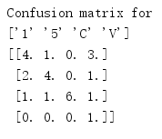
通过输出发现,对于V这个手势的识别和对1这个手势的识别存在高度的混淆情况。我查看了我训练的数据,发现存在的一些问题: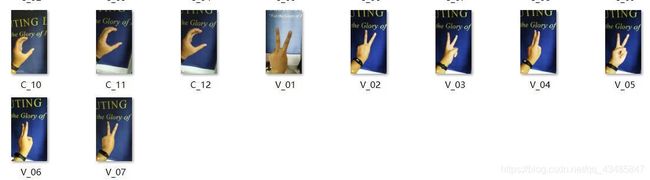
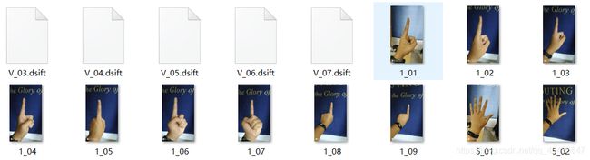
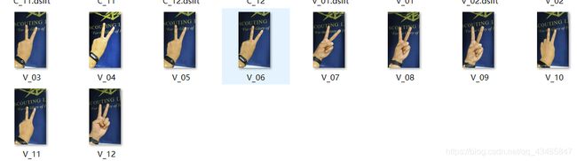
这两张图片是我训练的数据集,分别是V和1手势的训练数据。因为V手势的视角出现偏差导致和1的手势存在很大的相似度,所以我觉得可以是训练数据集的问题导致了准确度不高,V和1高度混淆。所以我使用另一组全新的手势V的数据作为测试集。
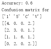
改成新数据集后,准确度和混淆矩阵如下:
发现准确度还是没有上升,于是我就改变test的测试数据集,删除了原来测试集中所以V手势的数据,使用一批全新的数据集测试,如下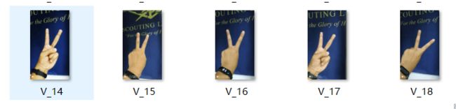
最后输出的准确度和混淆矩阵如下:
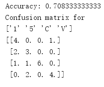
发现关于V和1手势的混淆不存在了,准确度也有所提升。所以我认为在测试时候准确度的高低一个是你测试数据的好坏,二是如果在训练数据足够多的情况下,可能测试数据的好坏对于准确度的影响会有所降低。