SPP、RFB和ASPP

                                      SPP、RFB和ASPP

   CNN中“金字塔”系列的结构块在深度学习诸多模型中发挥着重要的作用，个人认为有大类：“横向”并联金字塔结构(Google的Inception系列)和“纵向”特征金字塔（FPN）。前者输出的特征图融合了具有多种尺度感受野的特征；后者更侧重于是深层语义特征与浅层边缘特征的融合，这里主要学习一下前者的几个典型结构（SPP、RFB和ASPP）,这几种结构或许可以作为模型即插即用的组件，对于优化模型有帮助，更重要的是学到如何根据实际需求设计合适的模型。

1、SPP(Spatial Pyramid Pooling)

    空间金字塔池化在何凯明的SPPNet[1]中具有详尽的描述，解决的是如何在具有全连接层的网络中实现多尺度图像的输入，全连接层的输入是固定的，使用文中提及的SPP结构则可以实现无论输入特征图多大均能通过空间金字塔池化得到固定维度的神经元输入。其结构如下图所示：

                                                

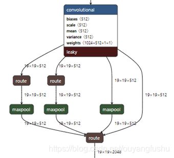
    如图所示，此处最后一层卷积conv5的输出维度256，按照图中三个并行的池化层计算则可得到256*（1+4+16）维的特征向量。在目标检测和语义分割的全卷积网络中，同样用到所谓的金字塔池化结构，但是结构上却有所不同，由于不需要展开成一个固定大小的一维向量，池化的Size则不一定是Sliding windows的形式（每个池化分支的对特征图划分的bins是固定不变的）。因此后续所谓的SPP都是修改后的结构。比如yolov3-spp[6]和yolov4[7]中的SPP结构仅仅是并联的池化层kernel size不用，输出特征图的大小则是相同的，如下图所示：

                                                              

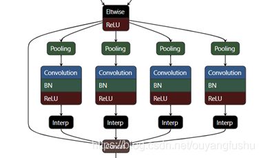
      另外在语义分割任务的PSPNet[8]中，则是普通的最大池化并联最后接一个上采样恢复到同样尺寸的特征图。如图所示输入特征图大小为60x60，池化的kernel size分别10，20,30,60，如下图所示。

                                               

 2、RFB(Receptive Field Block)

    论文[2]提出RFBNet目标检测网络，RFBNet是在SSD网络中引入Receptive Field Block (RFB) ，引入RFB的出发点通过模拟人类视觉的感受野加强网络的特征提取能力，在结构上RFB借鉴了Inception的思想，主要是在Inception的基础上加入了dilated卷积层（dilated convolution），从而有效增大了感受野（receptive field）。RFB结构对于增大轻量级目标检测网络的感受野很有帮助，并且不会引入过多的计算量和粗暴增加网络深度。原理部分论文[2]给出了一个比较形象的示意图，描述RFB中的dilated卷积层如何加持感受野金字塔的，一三五卷积核配合空洞卷积实现了感受野的增大及不同感受野特征图的融合。补充一下空洞卷积的卷积层感受野大小的计算式：

                                                                         

                                   

     论文[2]中的给出了RFB网络结构：

                                    

    论文[2]官方开源实现：https://github.com/ruinmessi/RFBNet

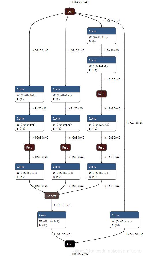
    另外 Github上的Ultra-Light-Fast-Generic-Face-Detector-1MB（https://github.com/Linzaer/Ultra-Light-Fast-Generic-Face-Detector-1MB）应该是一个应用RFB结构的较为火的的项目，超轻量超快速效果还不赖，其结构：

                                      

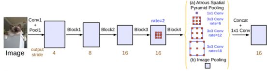
3、ASPP(atrous spatial pyramid pooling)[3,4,5]

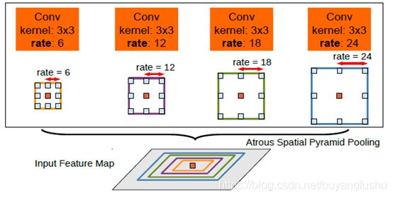
    RFBNet结构在Google的Incepetion系列的结构中引入了空洞卷积。同样用到了空洞卷积，其实 Google自家的ASPP（空洞空间卷积池化金字塔）也是能打的。ASPP最早是出现在语义分割网络DeepLabv2中，ASPP对所给定的输入以不同采样率的空洞卷积并行采样，相当于以多个比例捕捉图像的上下文，结构示意图如下

                                       

    论文[3]（DeepLabv2）中从语义分割的角度阐述了使用这个一结构的好处： 空洞卷积可以在不增加太多计算量的情况下增大滤波器的视野；空洞空间卷积池化金字塔可以增强模型对不同尺度分割目标的感知能力。

   DeepLabv3[4]的论文中通过实验作者发现：当膨胀率越大，卷积核中的有效权重越少，当膨胀率足够大时，只有卷积核最中间的权重有效，即退化成了1x1卷积核，并不能获取到全局的context信息；解决方案是在最后一个特征上使用了全局平均池化（global average pooling）（包含1x1卷积核，输出256个通道，正则化，通过bilinear上采样还原到对应尺度）,最后和其他并行的分支concat.

                                     

（已经用大老师的onnxsim merge了BN）的结构如下：

                              

1）Pytorch实现的不含BN版本代码：

class ASPPNOBN(nn.Module):
    def __init__(self, in_channel=512, depth=256):
        super(ASPPNOBN, self).__init__()
        self.mean = nn.AdaptiveAvgPool2d((1, 1))  # (1,1)means ouput_dim
        self.conv = nn.Conv2d(in_channel, depth, 1, 1)
        self.atrous_block1 = nn.Conv2d(in_channel, depth, 1, 1)
        self.atrous_block6 = nn.Conv2d(in_channel, depth, 3, 1, padding=6, dilation=6)
        self.atrous_block12 = nn.Conv2d(in_channel, depth, 3, 1, padding=12, dilation=12)
        self.atrous_block18 = nn.Conv2d(in_channel, depth, 3, 1, padding=18, dilation=18)
        self.conv_1x1_output = nn.Conv2d(depth * 5, depth, 1, 1)

    def forward(self, x):
        size = x.shape[2:]

        image_features = self.mean(x)
        image_features = self.conv(image_features)
        image_features = F.upsample(image_features, size=size, mode='bilinear')

        atrous_block1 = self.atrous_block1(x)
        atrous_block6 = self.atrous_block6(x)
        atrous_block12 = self.atrous_block12(x)
        atrous_block18 = self.atrous_block18(x)

        net = self.conv_1x1_output(torch.cat([image_features, atrous_block1, atrous_block6,
                                              atrous_block12, atrous_block18], dim=1))
        return net

2）Pytorch实现的BN版本代码(来自https://github.com/fregu856/deeplabv3)：

class ASPPBN(nn.Module):
    def __init__(self, in_planes=512,out_planes=256):
        super(ASPPBN, self).__init__()

        self.conv_1x1_1 = nn.Conv2d(in_planes, out_planes, kernel_size=1)
        self.bn_conv_1x1_1 = nn.BatchNorm2d(out_planes)

        self.conv_3x3_1 = nn.Conv2d(in_planes, out_planes, kernel_size=3, stride=1, padding=6, dilation=6)
        self.bn_conv_3x3_1 = nn.BatchNorm2d(out_planes)

        self.conv_3x3_2 = nn.Conv2d(in_planes, out_planes, kernel_size=3, stride=1, padding=12, dilation=12)
        self.bn_conv_3x3_2 = nn.BatchNorm2d(out_planes)

        self.conv_3x3_3 = nn.Conv2d(in_planes, out_planes, kernel_size=3, stride=1, padding=18, dilation=18)
        self.bn_conv_3x3_3 = nn.BatchNorm2d(out_planes)

        self.avg_pool = nn.AdaptiveAvgPool2d(1)

        self.conv_1x1_2 = nn.Conv2d(in_planes, out_planes, kernel_size=1,stride=1)
        self.bn_conv_1x1_2 = nn.BatchNorm2d(out_planes)

        self.conv_1x1_3 = nn.Conv2d(out_planes*5, out_planes, kernel_size=1) # (1280 = 5*256)
        self.bn_conv_1x1_3 = nn.BatchNorm2d(out_planes)


    def forward(self, feature_map):
        feature_map_h = feature_map.size()[2] # (== h/16)
        feature_map_w = feature_map.size()[3] # (== w/16)

        out_1x1 = F.relu(self.bn_conv_1x1_1(self.conv_1x1_1(feature_map))) # (shape: (batch_size, 256, h/16, w/16))
        out_3x3_1 = F.relu(self.bn_conv_3x3_1(self.conv_3x3_1(feature_map))) # (shape: (batch_size, 256, h/16, w/16))
        out_3x3_2 = F.relu(self.bn_conv_3x3_2(self.conv_3x3_2(feature_map))) # (shape: (batch_size, 256, h/16, w/16))
        out_3x3_3 = F.relu(self.bn_conv_3x3_3(self.conv_3x3_3(feature_map))) # (shape: (batch_size, 256, h/16, w/16))

        out_img = self.avg_pool(feature_map) # (shape: (batch_size, 512, 1, 1))
        out_img = F.relu(self.bn_conv_1x1_2(self.conv_1x1_2(out_img))) # (shape: (batch_size, 256, 1, 1))
        out_img = F.upsample(out_img, size=(feature_map_h, feature_map_w), mode="bilinear") # (shape: (batch_size, 256, h/16, w/16))

        out = torch.cat([out_1x1, out_3x3_1, out_3x3_2, out_3x3_3,out_img], 1) # (shape: (batch_size, 1280, h/16, w/16))
        out = F.relu(self.bn_conv_1x1_3(self.conv_1x1_3(out))) # (shape: (batch_size, 256, h/16, w/16))

        return out

参考资料：

[1]  He K , Zhang X , Ren S , et al. Spatial Pyramid Pooling in Deep Convolutional Networks for Visual Recognition[J]. 2014.

[2]  Liu S , Huang D , Wang Y . Receptive Field Block Net for Accurate and Fast Object Detection[J]. 2017.

[3]  Chen L C , Papandreou G , Kokkinos I , et al. DeepLab: Semantic Image Segmentation with Deep Convolutional Nets, Atrous Convolution, and Fully Connected CRFs[J]. IEEE Transactions on Pattern Analysis and Machine Intelligence, 2018, 40(4):834-848.

[4]  Chen L C , Papandreou G , Schroff F , et al. Rethinking Atrous Convolution for Semantic Image Segmentation[J]. 2017.

[5]  Ma X , Liu K , Ding C , et al. Encoder-decoder with multi-scale information fusion for semantic image segmentation[C]// Eleventh International Conference on Graphics and Image Processing. 2020.

[6]  Redmon J , Farhadi A . YOLOv3: An Incremental Improvement[J]. 2018.

[7]  Bochkovskiy A , Wang C Y , Liao H Y M . YOLOv4: Optimal Speed and Accuracy of Object Detection[J]. 2020.

[8]  Zhao H , Shi J , Qi X , et al. Pyramid Scene Parsing Network[J]. 2016.

9、https://blog.csdn.net/qq_36530992/article/details/102628455

10、https://www.jianshu.com/p/edbaa56d250d

11、https://blog.csdn.net/u014380165/article/details/81556769