CS224n课程Assignment1参考答案

$$Assignment\#1-solutionByJonariguez$$

所有的代码题目对应的代码已上传至github/CS224n/Jonariguez

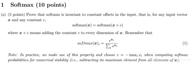
解：
$$softmax(\mathbf{x}{)}_i=\frac{e^{x_i}}{{\sum }_j{e}^{x_j}}=\frac{e^c{e}^{x_i}}{e^c{\sum }_j{e}^{x_j}}=\frac{e^{x_i+c}}{{\sum }_j{e}^{x_j+c}}=softmax(\mathbf{x}+c{)}_i$$
即
$$softmax(\mathbf{x})=softmax(\mathbf{x}+c)$$
证毕

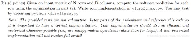
解：
直接在代码中利用numpy实现即可。注意要先从$x$中减去每一行的最大值，这样在保证结果不变的情况下，所有的元素不大于0，不会出现上溢出，从而保证结果的正确性。具体可参考 http://www.hankcs.com/ml/computing-log-sum-exp.html

def softmax(x):
   """Compute the softmax function for each row of the input x.

   It is crucial that this function is optimized for speed because
   it will be used frequently in later code. You might find numpy
   functions np.exp, np.sum, np.reshape, np.max, and numpy
   broadcasting useful for this task.

   Numpy broadcasting documentation:
   http://docs.scipy.org/doc/numpy/user/basics.broadcasting.html

   You should also make sure that your code works for a single
   N-dimensional vector (treat the vector as a single row) and
   for M x N matrices. This may be useful for testing later. Also,
   make sure that the dimensions of the output match the input.

   You must implement the optimization in problem 1(a) of the
   written assignment!

   Arguments:
   x -- A N dimensional vector or M x N dimensional numpy matrix.

   Return:
   x -- You are allowed to modify x in-place
   """
   orig_shape = x.shape

   if len(x.shape) > 1:
       # Matrix
       # 每行减去该行的最大值
       x = x-np.max(x,axis=1).reshape(x.shape[0],1)
       # 然后进行softmax计算
       x = np.exp(x)/np.sum(np.exp(x),axis=1).reshape(x.shape[0],1)
   else:
       # Vector
       x = x-np.max(x)
       x = np.exp(x)/np.sum(np.exp(x))

   assert x.shape == orig_shape
   return x

解：
$${\sigma }^{\prime }(x)=\frac{e^{-x}}{(1+e^{-x}{)}^2}=\frac{1}{1+e^{-x}}\cdot \frac{e^{-x}}{1+e^{-x}}=\sigma (x)\cdot (1-\sigma (x))$$

即$sigmoid$函数的求导可以由其本身来表示。

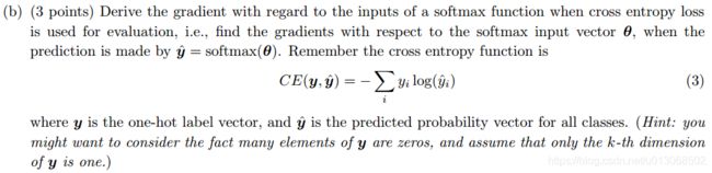
解：
我们知道真实标记$y$是one-hot向量，因此我们下面的推导都基于 $y_k=1$ ,且 $y_i=0,i̸=k$ ，即真实标记是 $k$ .

$$\frac{\partial CE(y,\hat{y})}{\partial \theta }=\frac{\partial CE(y,\hat{y})}{\partial \hat{y}}\cdot \frac{\partial \hat{y}}{\partial \theta }$$

其中：
$$\frac{\partial CE(y,\hat{y})}{\partial \hat{y}}=-\sum _i\frac{y_i}{{\hat{y}}_i}=-\frac{1}{{\hat{y}}_k}$$

接下来讨论 $\frac{\partial \hat{y}}{\partial \theta }$ :

1. $i=k$:
   $$\frac{\partial \hat{y}}{\partial {\theta }_k}=\frac{\partial }{\partial {\theta }_k}(\frac{e^{{\theta }_k}}{{\sum }_j{e}^{{\theta }_j}})={\hat{y}}_k\cdot (1-{\hat{y}}_k)$$

则：
$$\frac{\partial CE}{{\theta }_i}=\frac{\partial CE}{\partial \hat{y}}\frac{\partial \hat{y}}{{\theta }_i}=-\frac{1}{{\hat{y}}_k}\cdot {\hat{y}}_k\cdot (1-{\hat{y}}_k)={\hat{y}}_i-1$$

2. $i̸=k$:
   $$\frac{\partial \hat{y}}{\partial {\theta }_i}=\frac{\partial }{\partial {\theta }_i}(\frac{e^{{\theta }_k}}{{\sum }_j{e}^{{\theta }_j}})=-{\hat{y}}_i\cdot {\hat{y}}_k$$

则：
$$\frac{\partial CE}{{\theta }_i}=\frac{\partial CE}{\partial \hat{y}}\frac{\partial \hat{y}}{{\theta }_i}=-\frac{1}{{\hat{y}}_k}\cdot (-{\hat{y}}_i\cdot {\hat{y}}_k)={\hat{y}}_i$$

综上：
$$\frac{\partial CE(y,\hat{y})}{\partial {\theta }_i}=\{\begin{array}{ll}{\hat{y}}_i-1& i=k\\ {\hat{y}}_i& i̸=k\end{array}$$

或者：

$$\frac{\partial CE(y,\hat{y})}{\partial {\theta }_i}=\hat{y}-y$$

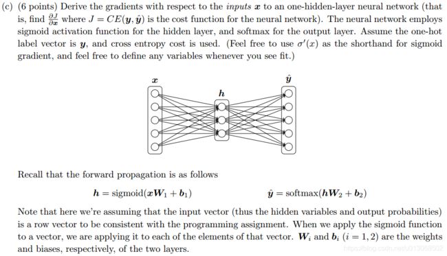
解：
首先设：$Z_1=x{W}_1+b_1$ 和 $Z_2=h{W}_2+b_2$，那么前向传播的顺序依次为：

$$Z_1=x{W}_1+b_1$$
$$h=sigmoid(Z_1)$$
$$Z_2=h{W}_2+b_2$$
$$\hat{y}=softmax(Z_2)$$
$$J=CE(y,\hat{y})=-\sum _i{y}_{i}log({\hat{y}}_i)$$

现在求$\frac{\partial J}{\partial x}$其实就是进行一次反向传播：
$${\delta }_1=\frac{\partial J}{\partial Z_2}=\hat{y}-y$$
$${\delta }_2=\frac{\partial J}{\partial Z_2}\cdot \frac{\partial Z_2}{\partial h}=(\hat{y}-y)\cdot \frac{\partial }{\partial x}(h{W}_2+b_2)={\delta }_1\cdot W_2^T$$
$${\delta }_3=\frac{\partial J}{\partial Z_2}\cdot \frac{\partial Z_2}{\partial h}\cdot \frac{\partial h}{\partial Z_1}={\delta }_2\cdot \frac{\partial (\sigma (Z_1))}{\partial Z_1}={\delta }_2\odot {\sigma }^{\prime }(Z_1)$$
$$\frac{\partial J}{\partial x}=\frac{\partial J}{\partial Z_2}\cdot \frac{\partial Z_2}{\partial h}\cdot \frac{\partial h}{\partial Z_1}\cdot \frac{\partial Z_1}{\partial x}={\delta }_3\cdot \frac{\partial }{\partial x}(x{W}_1+b_1)={\delta }_3\cdot W_1^T$$

解：
(1) 从输入层到隐藏层，全连接共$D_x\times H$个，即$W_1$，加上$H$个偏置项，共$D_x\times H+H$个。
(2) 从隐藏层到输出层，共$H\times D_y+D_y$个。
参数个数共：
$$(D_x\times H+H)+(H\times D_y+D_y)$$

def sigmoid(x):
    """
    Compute the sigmoid function for the input here.
    Arguments:
    x -- A scalar or numpy array.
    Return:
    s -- sigmoid(x)
    """
    # 按照sigmoid的函数定义即可
    s = 1/(1+np.exp(-x))
    return s


def sigmoid_grad(s):
    """
    Compute the gradient for the sigmoid function here. Note that
    for this implementation, the input s should be the sigmoid
    function value of your original input x.

    Arguments:
    s -- A scalar or numpy array.

    Return:
    ds -- Your computed gradient.
    """
    # s=sigmoid(x)
    # D(sigmoid(x))=sigmoid(x)*(1-sigmoid(x))=s*(1-s)
    ds = s*(1-s)
    return ds

def gradcheck_naive(f, x):
    """ Gradient check for a function f.

    Arguments:
    f -- a function that takes a single argument and outputs the
         cost and its gradients
    x -- the point (numpy array) to check the gradient at
    """
    rndstate = random.getstate()
    random.setstate(rndstate)
    fx, grad = f(x) # Evaluate function value at original point
    h = 1e-4        # Do not change this!

    # Iterate over all indexes in x
    it = np.nditer(x, flags=['multi_index'], op_flags=['readwrite'])
    while not it.finished:
        ix = it.multi_index
        # Try modifying x[ix] with h defined above to compute
        # numerical gradients. Make sure you call random.setstate(rndstate)
        # before calling f(x) each time. This will make it possible
        # to test cost functions with built in randomness later.

        ### YOUR CODE HERE:
        #根据导数的定义即可.但h->0,f(x+h)-f(x-h)/(2h)的极限。
        #这里采用f(x+h)-f(x)/h的精度不够
        x[ix] += h
        #先调用该函数，因为f的需要。另外，根据测试函数中f的定义可知，f(X)=sigma{xi^2}
        random.setstate(rndstate)
        new_f1 = f(x)[0]

        x[ix] -= 2*h
        random.setstate(rndstate)
        new_f2 = f(x)[0]

        delta = new_f1-new_f2
        numgrad = delta/(2*h)
        #将x变回来
        x[ix] += h
        ### END YOUR CODE
        # Compare gradients
        reldiff = abs(numgrad - grad[ix]) / max(1, abs(numgrad), abs(grad[ix]))
        if reldiff > 1e-5:
            print "Gradient check failed."
            print "First gradient error found at index %s" % str(ix)
            print "Your gradient: %f \t Numerical gradient: %f" % (
                grad[ix], numgrad)
            return

        it.iternext() # Step to next dimension

    print "Gradient check passed!"

def forward_backward_prop(data, labels, params, dimensions):
    """
    Forward and backward propagation for a two-layer sigmoidal network

    Compute the forward propagation and for the cross entropy cost,
    and backward propagation for the gradients for all parameters.

    Arguments:
    data -- M x Dx matrix, where each row is a training example.
    labels -- M x Dy matrix, where each row is a one-hot vector.
    params -- Model parameters, these are unpacked for you.
    dimensions -- A tuple of input dimension, number of hidden units
                  and output dimension
    """

    ### Unpack network parameters (do not modify)
    ofs = 0
    Dx, H, Dy = (dimensions[0], dimensions[1], dimensions[2])

    W1 = np.reshape(params[ofs:ofs+ Dx * H], (Dx, H))
    ofs += Dx * H
    b1 = np.reshape(params[ofs:ofs + H], (1, H))
    ofs += H
    W2 = np.reshape(params[ofs:ofs + H * Dy], (H, Dy))
    ofs += H * Dy
    b2 = np.reshape(params[ofs:ofs + Dy], (1, Dy))

    ### YOUR CODE HERE: forward propagation
    z1 = data.dot(W1)+b1
    h = sigmoid(z1)
    z2 = h.dot(W2)+b2
    y_ = softmax(z2)
    cost = np.sum(-np.log(y_[labels==1]))/data.shape[0]
    ### END YOUR CODE

    ### YOUR CODE HERE: backward propagation
    theta1 = (y_-labels)/data.shape[0]
    gradW2 = h.T.dot(theta1)
    gradb2 = np.sum(theta1,0)

    theta2 = theta1.dot(W2.T)
    theta3 = theta2*(sigmoid_grad(h))
    gradW1 = data.T.dot(theta3)
    gradb1 = np.sum(theta3,0)

    """
    总结：
        如果是有激活函数的，则反向传播的对激活函数求导之后，按元素相乘(*)
    """
    ### END YOUR CODE

    ### Stack gradients (do not modify)
    grad = np.concatenate((gradW1.flatten(), gradb1.flatten(),
        gradW2.flatten(), gradb2.flatten()))

    return cost, grad

解：
首先分析各个量的形状：$U=[u_1,u_2,...,u_W]\in d\times W$，$y,\hat{y}\in W\times 1$，其中$W$为词典大小，$d$为词向量的维度。
我们设：
$$\theta =\left[\begin{array}{c}{u}_1^T{v}_c\\ u_2^T{v}_c\\ ...\\ u_W^T{v}_c\end{array}\right]=U^T{v}_c\in W\times 1$$

则：
$${\hat{y}}_o=p(o|c)=\frac{exp(u_o^T{v}_c)}{{\sum }_{w=1}^{W}exp(u_w^T{v}_c)}=softmax(\theta {)}_o$$
$$\hat{y}=softmax(\theta )$$
那么：
$$\frac{\partial J}{\partial v_c}=\frac{\partial J}{\partial \theta }\cdot \frac{\partial \theta }{\partial v_c}=(\hat{y}-y)\cdot \frac{\partial }{\partial v_c}(U^T{v}_c)=U(\hat{y}-y)$$

解：
可以先对$U^T$求导：
$$\frac{\partial J}{\partial U^T}=\frac{\partial J}{\partial \theta }\cdot \frac{\partial \theta }{\partial U^T}=\frac{\partial J}{\partial \theta }\cdot \frac{\partial }{\partial U^T}(U^T{v}_c)=(\hat{y}-y)\cdot v_c^T$$

那么对 $U$ 求导的结果对上式转置即可：

$$\frac{\partial J}{\partial U}=((\hat{y}-y)\cdot v_c^T{)}^T=v_c\cdot (\hat{y}-y{)}^T$$
也可以表示为：
$$\frac{\partial J}{\partial U}=\{\begin{array}{ll}({\hat{y}}_w-1)\cdot v_c& w=o\\ {\hat{y}}_w\cdot v_c& w̸=o\end{array}$$

解：
首先应该知道：
$${\sigma }^{\prime }(x)=\sigma (x)\cdot (1-\sigma (x))$$
$$1-\sigma (x)=\sigma (-x)$$
已知：
$$J(o,v_c,U)=-log(\sigma (u_o^T{v}_c))-\sum _{k=1}^{K}log(\sigma (-u_k^T{v}_c))$$

直接求导即可：
$$\frac{\partial J}{\partial v_c}=-\frac{{\sigma }^{\prime }(u_o^T{v}_c)\cdot u_o}{\sigma (u_o^T{v}_c)}+\sum _{k=1}^K\frac{{\sigma }^{\prime }(-u_k^T{v}_c)\cdot u_k}{\sigma (-u_k^T{v}_c)}=(\sigma (u_o^T{v}_c)-1)u_o+\sum _{k=1}^K\sigma (u_k^T{v}_c)\cdot u_k$$
$$\frac{\partial J}{\partial u_k}=\{\begin{array}{ll}(\sigma (u_o^T{v}_c)-1)v_c& k=o\\ \sigma (u_k^T{v}_c)v_c& k̸=o\end{array}$$

解：
根据题目的提示可知，我们可以设$F(o,v_c)$为损失函数，等价于前面的$J_{softmax-CE}$或者$J_{neg-sample}$，而$J$对变量的求导我们前面已经做过，所以这里直接使用$\frac{\partial F(o,v_c)}{\partial ..}$代替即可，不用再进一步求导展开。
(1) skip-gram模型
$$J_{skip-gram}(wor{d}_{c-m..c+m})=\sum _{-m\le j\le m,j̸=0}F(w_{c+j},v_c)$$
$$\frac{\partial J}{\partial U}=\sum _{-m\le j\le m,j̸=0}\frac{\partial F(w_{c+j},v_c)}{\partial U}$$
$$\frac{\partial J}{\partial v_c}=\sum _{-m\le j\le m,j̸=0}\frac{\partial F(w_{c+j},v_c)}{\partial v_c}$$
$$\frac{\partial J}{\partial v_j}=0,j̸=c$$

(2) CBOW模型
因为CBOW模型是根据多个背景词预测一个中心词，又因为$F()$惩罚函数是形如(一个词，一个词)的形式，所以要把多个背景词变成一个词，那么一种有效的方式就是把这些背景词的词向量求平均便得到了一个词向量。
$$\hat{v}=\sum _{-m\le j\le m,j̸=0}{v}_{c+j}$$
$$J_{CBOW}(wor{d}_{c-m..c+m})=F(w_c,\hat{v})$$
那么：
$$\frac{\partial J}{\partial U}=\frac{\partial F(w_c,\hat{v})}{\partial U}$$
$$\frac{\partial J}{\partial v_c}=0,c\notin \{c-m,..,c-1,c+1,..c+m\}$$
$$\frac{\partial J}{\partial v_j}=\frac{\partial F(w_c,\hat{v})}{\partial \hat{v}}\cdot \frac{\partial \hat{v}}{\partial v_j}=\frac{\partial F(w_c,\hat{v})}{\partial v_j},c\in \{c-m,..,c-1,c+1,..c+m\}$$

def normalizeRows(x):
    """ Row normalization function

    Implement a function that normalizes each row of a matrix to have
    unit length.
    """
    ### YOUR CODE HERE
    F = np.apply_along_axis(lambda x:np.sqrt(x.T.dot(x)),axis=1,arr=x)
    x /= F.reshape(x.shape[0],1)
    ### END YOUR CODE
    return x

def softmaxCostAndGradient(predicted, target, outputVectors, dataset):
    """ Softmax cost function for word2vec models

    Implement the cost and gradients for one predicted word vector
    and one target word vector as a building block for word2vec
    models, assuming the softmax prediction function and cross
    entropy loss.

    Arguments:
    predicted -- numpy ndarray, predicted word vector (\hat{v} in
                 the written component)
    target -- integer, the index of the target word
    outputVectors -- "output" vectors (as rows) for all tokens
    dataset -- needed for negative sampling, unused here.

    Return:
    cost -- cross entropy cost for the softmax word prediction
    gradPred -- the gradient with respect to the predicted word
           vector
    grad -- the gradient with respect to all the other word
           vectors

    We will not provide starter code for this function, but feel
    free to reference the code you previously wrote for this
    assignment!
    """
    ### YOUR CODE HERE
    """
    重申一下：
        predicted       对应作业中的 v
        target          对应作用中的 I(y==1)
        outputVectors   对应作用中的 u (注意作业上的U是[u1,u2,..uW],维度为d*W,而这里是W*d的)
        gradPred        对应作用中的 dJ/dv_c
        grad            对应作用中的 dJ/du_w
    """
    v = predicted       # d*1
    u = outputVectors   # d*W
    y_ = softmax(u.dot(v))

    # cost是交叉熵
    cost = -np.log(y_[target])

    Y = y_.copy()
    Y[target] -= 1.0
    gradPred = u.T.dot(Y)
    grad     = np.outer(Y,v)
    ### END YOUR CODE
    return cost, gradPred, grad

def negSamplingCostAndGradient(predicted, target, outputVectors, dataset,
                               K=10):
    """ Negative sampling cost function for word2vec models

    Implement the cost and gradients for one predicted word vector
    and one target word vector as a building block for word2vec
    models, using the negative sampling technique. K is the sample
    size.

    Note: See test_word2vec below for dataset's initialization.

    Arguments/Return Specifications: same as softmaxCostAndGradient
    """

    # Sampling of indices is done for you. Do not modify this if you
    # wish to match the autograder and receive points!
    indices = [target]
    indices.extend(getNegativeSamples(target, dataset, K))

    ### YOUR CODE HERE
    v = predicted
    u = outputVectors
    # indices[0]里面保存的是target，即正确的背景词，对用作用中的o，而indices[1:]都是噪声词，通过负采样得到的
    grad = np.zeros(u.shape)
    gradPred = np.zeros(v.shape)
    cost = 0

    # 先算正例的损失和梯度
    val = sigmoid(u[target].dot(v))-1
    cost -= np.log(val+1)

    gradPred += val*u[target]
    grad[target] = val*v

    # 然后再算负例，注意利用了:1-sigmoid(-x)=sigmoid(x)
    for samp in indices[1:]:
        val = sigmoid(u[samp].dot(v))
        gradPred += val*u[samp]
        grad[samp] += val*v
        cost -= np.log(1-val)

    # cost = -np.log(sigmoid(u[indices[0]].dot(v)))-np.sum(np.log(sigmoid(-u[indices[1:]].dot(v))),0)
    #
    # rea_idx = target
    # neg_idx = indices[1:]
    # gradPred = sigmoid(sigmoid(u[rea_idx].dot(v))-1)*u[rea_idx]+np.sum((1-sigmoid(-u[neg_idx].dot(v)))*u[neg_idx],0)
    # grad =
    ### END YOUR CODE

    return cost, gradPred, grad

def skipgram(currentWord, C, contextWords, tokens, inputVectors, outputVectors,
             dataset, word2vecCostAndGradient=softmaxCostAndGradient):
    """ Skip-gram model in word2vec

    Implement the skip-gram model in this function.

    Arguments:
    currrentWord -- a string of the current center word
    C -- integer, context size
    contextWords -- list of no more than 2*C strings, the context words
    tokens -- a dictionary that maps words to their indices in
              the word vector list
    inputVectors -- "input" word vectors (as rows) for all tokens
    outputVectors -- "output" word vectors (as rows) for all tokens
    word2vecCostAndGradient -- the cost and gradient function for
                               a prediction vector given the target
                               word vectors, could be one of the two
                               cost functions you implemented above.

    Return:
    cost -- the cost function value for the skip-gram model
    grad -- the gradient with respect to the word vectors
    """
    """
    currrentWord        中心词
    contextWords        背景词
    inputVectors        初始化的词向量v
    outputVectors       训练好的词向量u
    """
    cost = 0.0
    gradIn = np.zeros(inputVectors.shape)
    gradOut = np.zeros(outputVectors.shape)

    ### YOUR CODE HERE
    center_id = tokens[currentWord]
    # 拿到中心词的中心词向量，对应作业中的v_c
    v = inputVectors[center_id]

    for context in contextWords:
        context_id = tokens[context]
        # 真正的背景词下标为context_id --> target
        c_cost,c_gradin,c_gradout = word2vecCostAndGradient(v,context_id,outputVectors,dataset)
        cost += c_cost
        # 对于v_c的梯度要增加在center_id上，而不是gradIn += c_gradin
        gradIn[center_id] += c_gradin
        gradOut += c_gradout
    ### END YOUR CODE

    return cost, gradIn, gradOut

def sgd(f, x0, step, iterations, postprocessing=None, useSaved=False,
        PRINT_EVERY=10):
    """ Stochastic Gradient Descent

    Implement the stochastic gradient descent method in this function.

    Arguments:
    f -- the function to optimize, it should take a single
         argument and yield two outputs, a cost and the gradient
         with respect to the arguments
    x0 -- the initial point to start SGD from
    step -- the step size for SGD
    iterations -- total iterations to run SGD for
    postprocessing -- postprocessing function for the parameters
                      if necessary. In the case of word2vec we will need to
                      normalize the word vectors to have unit length.
    PRINT_EVERY -- specifies how many iterations to output loss

    Return:
    x -- the parameter value after SGD finishes
    """

    # Anneal learning rate every several iterations
    ANNEAL_EVERY = 20000
    if useSaved:
        start_iter, oldx, state = load_saved_params()
        if start_iter > 0:
            x0 = oldx
            step *= 0.5 ** (start_iter / ANNEAL_EVERY)
        if state:
            random.setstate(state)
    else:
        start_iter = 0

    x = x0

    if not postprocessing:
        postprocessing = lambda x: x

    expcost = None

    for iter in xrange(start_iter + 1, iterations + 1):
        # Don't forget to apply the postprocessing after every iteration!
        # You might want to print the progress every few iterations.

        cost = None
        ### YOUR CODE HERE
        cost,f_grad = f(x)
        # 根据梯度来更新x，也就是下降x
        x -= step*f_grad
        x = postprocessing(x)

        ### END YOUR CODE

        if iter % PRINT_EVERY == 0:
            # 滑动
            if not expcost:
                expcost = cost
            else:
                expcost = .95 * expcost + .05 * cost
            print "iter %d: %f" % (iter, expcost)

        if iter % SAVE_PARAMS_EVERY == 0 and useSaved:
            save_params(iter, x)

        if iter % ANNEAL_EVERY == 0:
            step *= 0.5

    return x

解：
我本地共训练了5+个小时。
输出的结果为：

解：
按题目要求实现即可。

def getSentenceFeatures(tokens, wordVectors, sentence):
    """
    Obtain the sentence feature for sentiment analysis by averaging its
    word vectors
    """

    # Implement computation for the sentence features given a sentence.

    # Inputs:
    # tokens -- a dictionary that maps words to their indices in
    #           the word vector list
    # wordVectors -- word vectors (each row) for all tokens
    # sentence -- a list of words in the sentence of interest

    # Output:
    # - sentVector: feature vector for the sentence

    sentVector = np.zeros((wordVectors.shape[1],))

    ### YOUR CODE HERE
    """
    给一个句子，然后该句子的对应的特征向量为：句子中所有单词的词向量的平均
    """
    for word in sentence:
        word_vec = wordVectors[tokens[word]]
        sentVector += word_vec
    sentVector = sentVector/len(sentence)
    ### END YOUR CODE

    assert sentVector.shape == (wordVectors.shape[1],)
    return sentVector

解： 引入正则化可以降低模型复杂度，进而避免过拟合，以提升泛化能力。

解： 注意是按照模型的验证集准确率来选择最优模型。

def getRegularizationValues():
    """Try different regularizations

    Return a sorted list of values to try.
    """
    values = None   # Assign a list of floats in the block below
    ### YOUR CODE HERE
    """
    应该是正则化系数，相当于lambda或者1/lambda
    """
    # 参考了一下别人的写法
    values = np.logspace(-4, 2, num=100, base=10)
    ### END YOUR CODE
    return sorted(values)

def chooseBestModel(results):
    """Choose the best model based on parameter tuning on the dev set

    Arguments:
    results -- A list of python dictionaries of the following format:
        {
            "reg": regularization,
            "clf": classifier,
            "train": trainAccuracy,
            "dev": devAccuracy,
            "test": testAccuracy
        }

    Returns:
    Your chosen result dictionary.
    """
    bestResult = None

    ### YOUR CODE HERE
    """
    题目要求是：Choose the best model based on parameter tuning on the dev set
    也就是根据dev set验证集的准确率来选择最佳模型
    所以就选择模型列表中dev对应的最大的那个即可
    max()函数利用key参数来决定选择依据
    """
    bestResult = max(results,key=lambda x: x['dev'])
    ### END YOUR CODE

    return bestResult

解： 我的本地答案：
(1) 使用自己训练的词向量的结果

Best regularization value: 7.05E-04
Test accuracy (%): 30.361991
dev accuracy (%): 32.698

(2) 使用预训练的词向量的结果

Best regularization value: 1.23E+01
Test accuracy (%): 37.556561
dev accuracy (%): 37.148

使用预训练的词向量的效果更好的原因：

• 其数据量大。
• 训练充分。
• 其采用的为GloVe,该模型利用全局的信息。
• 维度高。

解：

解释：随着正则化因子的增大，最终所得的模型越简单，拟合能力差，出现欠拟合，导致两者的准确率下降。

解：