Bag of features 图像特征词典原理及实现

1、原理

首先来了解一下基本流程，根据流程介绍原理：

1. 特征提取
2. 学习 “视觉词典（visual vocabulary）”
3. 针对输入特征集，根据视觉词典进行量化
4. 把输入图像，根据TF-IDF转化成视觉单词（visual words）的频率直方图
5. 构造特征到图像的倒排表，通过倒排表快速索引相关图像
6. 根据索引结果进行直方图匹配

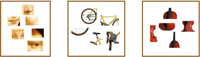
1.特征提取

特征提取就是通过我们常用的sifi方法，提取图像的特征

2. 学习 “视觉词典”

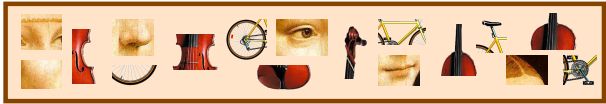
对于一个庞大的数据集，可以通过聚类算法构建出视觉词典，聚类是实现 visual vocabulary /codebook的关
键，最常用的就是K-means算法，算法流程:
• 随机初始化 K 个聚类中心
• 重复下述步骤直至算法收敛:

1. 对应每个特征，根据距离关系赋值给某个中心/类别
2. 对每个类别，根据其对应的特征集重新计算聚类中心

3. 针对输入特征集，根据视觉词典进行量化

对于输入特征，量化的过程是将该特征映射到距离其最接近的视觉单词，并实现计数。
这里要注意选择视觉词典的规模。太少：视觉单词无法覆盖所有可能出现的情况；太多：计算量大，容易过拟合。

4. 把输入图像，根据TF-IDF转化成视觉单词（visual words）的频率直方图

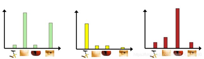
给定输入图像的BOW直方图, 在数据库中查找 k 个最近邻的图像
对于图像分类问题，可以根据这k个近邻图像的分类标签，投票获得分类结果
当训练数据足以表述所有图像的时候，检索/分类效果良好

5. 构造特征到图像的倒排表，通过倒排表快速索引相关图像

利用倒排表可以快速使用反转文件进行计算新图像与数据库中所有图像之间的相似性

6. 根据索引结果进行直方图匹配

2、实现

首先测试一下官方数据（first1000）中的1000张图像集

1.生成代码所需要的模型文件

生成视觉词典：

# -*- coding: utf-8 -*-
import pickle
from PCV.imagesearch import vocabulary
from PCV.tools.imtools import get_imlist
from PCV.localdescriptors import sift
##要记得将PCV放置在对应的路径下
#获取图像列表
imlist = get_imlist('D:/Visual_Studio_Code/data/first1000/') ###要记得改成自己的路径
nbr_images = len(imlist)
#获取特征列表
featlist = [imlist[i][:-3]+'sift' for i in range(nbr_images)]
#提取文件夹下图像的sift特征
for i in range(nbr_images):
    sift.process_image(imlist[i], featlist[i])
#生成词汇
voc = vocabulary.Vocabulary('ukbenchtest')
voc.train(featlist, 1000, 10)
#保存词汇
# saving vocabulary
with open(r'D:\Visual_Studio_Code\data\first1000\vocabulary.pkl', 'wb') as f:
    pickle.dump(voc, f)
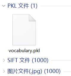
print ('vocabulary is:', voc.name, voc.nbr_words)

对应1000张图像生成了1000个sift文件，并且生成了视觉词典

2.将模型数据导入数据库

在python\Lib文件夹之下可以看到一个sqlite3的包，说明python3自带数据库包，不需要安装pysqlite库，所以需要更改PCV\imagesearch中的imagesearch.py文件第三行为from sqlite3 import dbapi2 as sqlite

# -*- coding: utf-8 -*-
import pickle
from PCV.imagesearch import imagesearch
from PCV.localdescriptors import sift
from sqlite3 import dbapi2 as sqlite
from PCV.tools.imtools import get_imlist
##要记得将PCV放置在对应的路径下
#获取图像列表
imlist = get_imlist('D:/Visual_Studio_Code/data/first1000/')##记得改成自己的路径
nbr_images = len(imlist)
#获取特征列表
featlist = [imlist[i][:-3]+'sift' for i in range(nbr_images)]
# load vocabulary
#载入词汇
with open(r'D:\Visual_Studio_Code\data\first1000\vocabulary.pkl', 'rb') as f:
    voc = pickle.load(f)
#创建索引
indx = imagesearch.Indexer('testImaAdd.db',voc)
indx.create_tables()
# go through all images, project features on vocabulary and insert
#遍历所有的图像，并将它们的特征投影到词汇上
for i in range(nbr_images)[:1000]:
    locs,descr = sift.read_features_from_file(featlist[i])
    indx.add_to_index(imlist[i],descr)
# commit to database
#提交到数据库
indx.db_commit()
con = sqlite.connect('testImaAdd.db')
print (con.execute('select count (filename) from imlist').fetchone())
print (con.execute('select * from imlist').fetchone())

运行后发现在代码文件夹之下生成了一个数据库文件

3.测试

这一部分其实个人代码还没有调通，在imagesearch.py出现了各种问题，包括str与bytes-like的类型不兼容（imagesearch.py中的第97行删除原来的str）

sort()函数中缺少了cmp之类的问题（暂时没解决，之后的问题还不懂）。为了不影响实验进度，我先使用学弟调好的包进行实验，之后再慢慢调试自己的代码。

# -*- coding: utf-8 -*-
import pickle
from PCV.localdescriptors import sift
from PCV.imagesearch import imagesearch
from PCV.geometry import homography
from PCV.tools.imtools import get_imlist

# load image list and vocabulary
#载入图像列表
imlist = get_imlist('first1000/')
nbr_images = len(imlist)
#载入特征列表
featlist = [imlist[i][:-3]+'sift' for i in range(nbr_images)]

#载入词汇
with open('first1000/vocabulary.pkl', 'rb') as f:
    voc = pickle.load(f)

src = imagesearch.Searcher('testImaAdd.db',voc)

# index of query image and number of results to return
#查询图像索引和查询返回的图像数
q_ind = 0
nbr_results = 20

# regular query
# 常规查询(按欧式距离对结果排序)
res_reg = [w[1] for w in src.query(imlist[q_ind])[:nbr_results]]
print ('top matches (regular):', res_reg)

# load image features for query image
#载入查询图像特征
q_locs,q_descr = sift.read_features_from_file(featlist[q_ind])
fp = homography.make_homog(q_locs[:,:2].T)

# RANSAC model for homography fitting
#用单应性进行拟合建立RANSAC模型
model = homography.RansacModel()
rank = {}

# load image features for result
#载入候选图像的特征
for ndx in res_reg[1:]:
    locs,descr = sift.read_features_from_file(featlist[ndx])  # because 'ndx' is a rowid of the DB that starts at 1
    # get matches
    matches = sift.match(q_descr,descr)
    ind = matches.nonzero()[0]
    ind2 = matches[ind]
    tp = homography.make_homog(locs[:,:2].T)
    # compute homography, count inliers. if not enough matches return empty list
    try:
        H,inliers = homography.H_from_ransac(fp[:,ind],tp[:,ind2],model,match_theshold=4)
    except:
        inliers = []
    # store inlier count
    rank[ndx] = len(inliers)

# sort dictionary to get the most inliers first
sorted_rank = sorted(rank.items(), key=lambda t: t[1], reverse=True)
res_geom = [res_reg[0]]+[s[0] for s in sorted_rank]
print ('top matches (homography):', res_geom)

# 显示查询结果
imagesearch.plot_results(src,res_reg[:8]) #常规查询
imagesearch.plot_results(src,res_geom[:8]) #重排后的结果

这里主要是对比两种查询方式：

1. 常规查询
2. 用单应性进行拟合建立RANSAC模型

在这一实验下两种方式的结果一致，都成功找到了和第一张图片内容一个类型的数据集：

3、总结

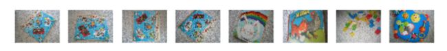
用自己的数据时由于数据收集较难，找了一个20张图片的数据集进行测试，第一次发现效果很差，基本没有匹配成功的，第二次增加了数据集中与第一张图片同类型的图片，共有8张（感觉有点作弊），发现效果有所改善，如下图（第四第六错误，其他都对）：

但是由于数据集实在太小，加上图片占比重较大（20张有8张），所以结果感觉不太能证明算法的正确性。
两种查询方式在多次实验中均展示了相同的结果，运行速度感觉没有太大差异（可能和数据集有关）。
通过改变数据集可以发现有两种情况测试结果相对好一些：

1. 特征明显的图片
2. 数据集中出现次数较多的图片

但是以上总结还是建立在个人的推测上，因为数据集确实太小，还需要更多次测试才能得出正确结论