泰坦尼克号之预测幸存人数

 

数据链接：链接：https://pan.baidu.com/s/1barfJ-nSzWL0yHOQjpRCSw   提取码：p3ga 

1.数据说明

首先说明一下各个字段的意思：

PassengerId	Survived	Pclass	Name	Sex	Age	SibSp	Parch	Ticket	Fare	Cabin	Embarked
1	0	3	Braund, Mr. Owen Harris	male	22	1	0	A/5 21171	7.25		S
2	1	1	Cumings, Mrs. John Bradley (Florence Briggs Thayer)	female	38	1	0	PC 17599	71.2833	C85	C

Passengerld：乘客编号，这是个顺序编号，用来唯一标致乘客

Survived：1表示幸存下来，0表示遇难，这应该是我们要预测的数据

Pclass：仓位等级（看过电影的估计都知道，高仓位的在上面，能更快的到达甲板）

Name：乘客姓名

Sex：性别（看过电影的人都知道，船长让妇女和儿童先上救生艇）

Age:年龄（儿童会先上救生艇，年轻的幸存概率大一点）

SibSp：兄弟姐妹在船上的数量

Parch：父母在船上的数量

Ticket：票号

Fare：票价

Cabin：乘客所在的船舱号

Embarked：乘客的等船口（需要转换为数值型数据）

 

2.数据分析

首先导入所需要用到的库

import numpy as np
import pandas as pd
import matplotlib.pyplot as plt

通过pandas库加载测试集数据和训练集数据

train=pd.read_csv("titanic_train.csv")
test=pd.read_csv("titanic_test.csv")

查看数据的前5行，head()里面如果不填，默认为5

print(train.head())

   PassengerId  Survived  Pclass    ...        Fare Cabin  Embarked
0            1         0       3    ...      7.2500   NaN         S
1            2         1       1    ...     71.2833   C85         C
2            3         1       3    ...      7.9250   NaN         S
3            4         1       1    ...     53.1000  C123         S
4            5         0       3    ...      8.0500   NaN         S

通过info()去查看各数据的字段类型及缺失情况

print(train.info())

得到的结果如下，可以很明显的看到，Age和Cabin字段缺失了挺多的，Embark也缺失了两个，不过这个无伤大雅，用均值补上就可以了

RangeIndex: 891 entries, 0 to 890
Data columns (total 12 columns):
PassengerId    891 non-null int64
Survived       891 non-null int64
Pclass         891 non-null int64
Name           891 non-null object
Sex            891 non-null object
Age            714 non-null float64
SibSp          891 non-null int64
Parch          891 non-null int64
Ticket         891 non-null object
Fare           891 non-null float64
Cabin          204 non-null object
Embarked       889 non-null object
dtypes: float64(2), int64(5), object(5)

通过describe()函数去统计各个字段的一些数

print(train.describe())

count(个数) mean(平均数) std(标准差),最小最大值......

       PassengerId    Survived     ...           Parch        Fare
count   891.000000  891.000000     ...      891.000000  891.000000
mean    446.000000    0.383838     ...        0.381594   32.204208
std     257.353842    0.486592     ...        0.806057   49.693429
min       1.000000    0.000000     ...        0.000000    0.000000
25%     223.500000    0.000000     ...        0.000000    7.910400
50%     446.000000    0.000000     ...        0.000000   14.454200
75%     668.500000    1.000000     ...        0.000000   31.000000
max     891.000000    1.000000     ...        6.000000  512.329200

对数据有了大致的了解之后，该思考如何处理数据了

首先，对缺失值的处理，Age字段准备用均值进行填充，fillna()，括号里为填充的值，如果写fillna(0),则填充的为0

train['Age']=train['Age'].fillna(train['Age'].median())

丢弃无用的字段（姓名、兄弟姐妹在穿上的数量、乘客票号、乘客所在的船舱号）,axis=1表示竖轴，inplace表示源数据改变

train.drop(['Name','SibSp','Ticket','Cabin','Parch','PassengerId'],axis=1,inplace=True)

然后我们使用可视化的方法，找出前面几个字段和是否幸存之间的联系

处理年龄，咱们用箱型图看一下

plt.style.use('ggplot')
fig=plt.figure(figsize=(5,7))
sns.boxplot(train['Age'],orient='v')
plt.ylabel('age')
plt.tight_layout()
plt.show()

发现大部分位于20-35之间

我们再用小提琴图来看一下各个年龄的分布情况

再看年龄、仓位等级、登船入口和幸存之间的关系，通过seaborn来作图

从中可以看到女性获救的比例要稍微大点，这也符合当时船长的命令；高等级仓获救的比例也要大一点；从登船港口发现，S登船的遇难比例要多一点

column=['Pclass','Sex','Embarked']
for i in range(3):
    plt.subplot(1,3,i+1)
    sns.countplot(x=column[i],hue='Survived',data=train)
plt.show()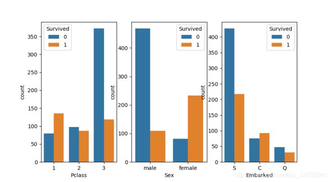

然后我们对特征的年龄进行分类，child小于12：youth 小于30：adult 小于60：old 小于75：tooold 大于75,其他的null

train['Age']=train['Age'].map(lambda x: 'child' if x<12 else 'youth' if x<30 else 'adlut' if x<60 else 'old' if x<75 else 'tooold' if x>=75 else 'null')

再通过print(train['Age'])查询一下结果

0    youth
1    adlut
2    youth
3    adlut
4    adlut
Name: Age, dtype: object

由于模型只能处理数值型数据，所以我们要将上一句前加个#号，重新处理Age这个字段，将之转为数值型数据,在此提供两种转化成数值型的方法

法一：

train['Age']=train['Age'].map(lambda x: 0 if x<12 else 1 if x<30 else 2 if x<60 else 3 if x<75 else 4 if x>=75 else 5)

法二：

labels=train['Age'].unique().tolist()
train['Age']=train['Age'].apply(lambda n:labels.index(n))

同样的，Sex字段为female,male；我们也要将它转化成数值型数据

train['Sex']=train['Sex'].map(lambda x:0 if x=='male' else 1)

处理登船港口数据，将之变为数值型

label为['S', 'C', 'Q', nan]，变为数值型[0,1,2,3]

labels=train['Embarked'].unique().tolist()
train['Embarked']=train['Embarked'].apply(lambda n:labels.index(n))

3.模型构建-决策树

1.原始模型

首先从sklearn库里引入专门划分数据的包：train_test_split，以8：2的方式区切分训练数据集，一部分为训练集，一部分为测试集，打印出来的结果为训练集有712行7列，测试集有179行7列。

from sklearn.model_selection import train_test_split
y=train['Survived'].values
x=train.drop(['Survived'],axis=1).values

x_train,x_test,y_train,y_test=train_test_split(x,y,test_size=0.2)
print("x_train:{0};x_test:{1}".format(x_train.shape,x_test.shape))

x_train:(712, 6);x_test:(179, 6)

接下来，就开始使用决策树模型对数据进行拟合，得到的结果发现和测试集的拟合度为78.7%

from sklearn.tree import DecisionTreeClassifier

clf=DecisionTreeClassifier()
clf.fit(x_train,y_train)

train_score=clf.score(x_train,y_train)
test_score=clf.score(x_test,y_test)
print("train_score:{0},test_score:{1}".format(train_score,test_score))

train_score:1.0,test_score:0.7877094972067039

从输出数据中看到，对训练集的拟合度是100%，但是对测试集的数据是78%，很明显，这是过拟合的特征，对于决策树模型而言，解决过拟合有两种方法：前剪枝和后剪枝。不过很抱歉，sklearn不支持后剪枝，所以我们只能前剪枝，通过max_depth和min_impurity(信息熵或基尼不纯度的阈值）区限定决策树分裂的深度来消除过拟合。

2.优化模型参数

2.1 max_depth

对模型的深度作出限定，生成一个2-11的列表depths，通过循环的方式代入决策树模型里,分别看看各个深度所得出的对测试集的分数是多高，生成一个te_score的列表，然后找出拟合值最大的一个，并且找到对应的决策树的深度max_depth的值，可以从结果中看到，max_depth为6的时候，有最大的预测值84%

def cv_score(d):
    clf=DecisionTreeClassifier(max_depth=d)
    clf.fit(x_train,y_train)

    train_score=clf.score(x_train,y_train)
    test_score=clf.score(x_test,y_test)
    print("train_score:{0},test_score:{1}".format(train_score,test_score))
    return (train_score,test_score)

depths=np.arange(2,12)
scores=[cv_score(d) for d in depths ]
tr_score=[s[0] for s in scores]
te_score=[s[1] for s in scores]
print(scores)

best_index=np.argmax(te_score)
best_score=np.max(te_score)
index=depths[best_index]
print(index,best_score)

train_score:0.7879213483146067,test_score:0.8044692737430168
train_score:0.824438202247191,test_score:0.8212290502793296
train_score:0.8342696629213483,test_score:0.8212290502793296
train_score:0.8455056179775281,test_score:0.8212290502793296
train_score:0.8651685393258427,test_score:0.8435754189944135
train_score:0.8904494382022472,test_score:0.8044692737430168
train_score:0.9101123595505618,test_score:0.8212290502793296
train_score:0.9283707865168539,test_score:0.8044692737430168
train_score:0.949438202247191,test_score:0.7821229050279329
train_score:0.9606741573033708,test_score:0.7932960893854749
[(0.7879213483146067, 0.8044692737430168), (0.824438202247191, 0.8212290502793296), (0.8342696629213483, 0.8212290502793296), (0.8455056179775281, 0.8212290502793296), (0.8651685393258427, 0.8135754589944135), (0.8904494382022472, 0.8044692737430168), (0.9101123595505618, 0.8435754189944135), (0.9283707865168539, 0.8044692737430168), (0.949438202247191, 0.7821229050279329), (0.9606741573033708, 0.7932960893854749)]
8 0.8435754189944135

我们也可以使用可视化的方法，更直观的观察max_depth和预测值的变化规律

#用来正常显示中文图例
plt.rcParams['font.sans-serif']=['SimHei']
plt.rcParams['axes.unicode_minus']=False

plt.figure(figsize=(6,4)) #figsize：限定图片的长和宽
plt.grid() #拥有网格
plt.plot(depths,te_score,'r--',label=u'测试集')
plt.plot(depths,tr_score,'g-',label=u'训练集')
plt.xlabel("max_depth")
plt.ylabel("value")
plt.legend() #显示label图例
plt.show()

从图中可以看出，当最大深度是8的时候测试集的预测准确度最高，但是我们要注意的是，由于数据切分的时候是随机切分的，所以每次切分的数据都是不一样的，由此得到的模型也不一样，因此当你重复运行程序的时候，可能有最大预测值的时候，并不是8，而是其他的值，也要注意一下。

2.2 min_impurity_split

2.3 criterion='gini'或'entropy'

以上两种调试方案就请读者自行完成啦，方法和max_depth完全一样

3. 缺点分析和解决方案

第一，数据不稳定，每次随机选取的训练集和测试集都不一样

第二，不能一次选择多个参数同时进行优化

解决方案：第一：多次计算，求平均值

                  第二：优化代码，使用GridSearchCV类，去组合各个参数

from sklearn.tree import DecisionTreeClassifier
from sklearn.model_selection import GridSearchCV

thresholds=np.linspace(0,0.5,50)
#设置参数矩阵
param_grid={'min_impurity_split':thresholds}
clf=GridSearchCV(DecisionTreeClassifier(),param_grid,cv=5)
clf.fit(x,y)
print("min_impurity_split:{0}\nbest score:{1}".format(clf.best_params_,clf.best_score_))

笔者在计算机上的输出结果如下：

min_impurity_split:{'min_impurity_split': 0.2040816326530612}
best score:0.8215488215488216

其中最关键的一个参数是param_grid，这是一个字典，同样也可以放入其他特征（如max_depth)，另一个关键参数是cv：表示把数据集平均分成5份，其中一份作为测试集，最终得出的最优参数和最终结果保存在clf.best_params_和clf.best_score_里

接下来看一下如何在多组参数间选择最优参数：(新版python，已经将min_impurity_split换成min_impurity_decrease了

from sklearn.tree import DecisionTreeClassifier
from sklearn.model_selection import GridSearchCV

entropy_thresholds=np.linspace(0,1,50)
gini_thresholds=np.linspace(0,0.5,50)
#设置参数矩阵
param_grid=[{'criterion':['entropy'],'min_impurity_decrease':entropy_thresholds},
            {'criterion':['gini'],'min_impurity_decrease':gini_thresholds},
            {'max_depth':range(2,10)},
            {'min_samples_split':range(2,30,2)}]

clf=GridSearchCV(DecisionTreeClassifier(),param_grid,cv=5)
clf.fit(x,y)
print("min_impurity_split:{0}\nbest score:{1}".format(clf.best_params_,clf.best_score_))

结果如下：

min_impurity_split:{'criterion': 'gini', 'min_impurity_split': 0.21428571428571427}
best score:0.8181818181818182