Noncentral chi-squared distribution
Noncentral chi-squared distribution
|
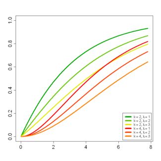
Probability density function
 |
|
|
Cumulative distribution function
 |
|
| Parameters |
 non-centrality parameter non-centrality parameter |
|---|---|
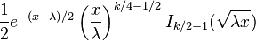
| Support | 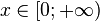 |
 |
|
| CDF | 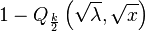 with Marcum Q-function with Marcum Q-function  |
| Mean |  |
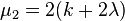
| Variance |  |
| Skewness | 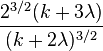 |
| Ex. kurtosis |  |
| MGF |  |
| CF |  |
 degrees of freedom
In probability theory and statistics, the noncentral chi-squared or noncentral  distribution is a generalization of the chi-squared distribution. This distribution often arises in the power analysis of statistical tests in which the null distribution is (perhaps asymptotically) a chi-squared distribution; important examples of such tests are the likelihood ratio tests.
Contents
[hide]- 1 Background
- 2 Definition
- 3 Properties
- 3.1 Moment generating function
- 3.2 Moments
- 3.3 Cumulative distribution function
- 3.3.1 Approximation
- 3.4 Differential equation
- 4 Derivation of the pdf
- 5 Related distributions
- 5.1 Transformations
- 6 Occurrences
- 6.1 Use in tolerance intervals
- 7 Notes
- 8 References
- 9 External Links
Background[edit]
Let ( ,
, 

 ) be k independent, normally distributed random variables with means
  and unit variances. Then the random variable

is distributed according to the noncentral chi-squared distribution. It has two parameters:  which specifies the number of degrees of freedom (i.e. the number of
  ), and
  which is related to the mean of the random variables by:

is sometimes called the noncentrality parameter. Note that some references define in other ways, such as half of the above sum, or its square root.
This distribution arises in multivariate statistics as a derivative of the multivariate normal distribution. While the central chi-squared distribution is the squared norm of a random vector with  distribution (i.e., the squared distance from the origin of a point taken at random from that distribution), the non-central is the squared norm of a random vector with
  distribution. Here
  is a zero vector of length k,
  and
and  is theidentity matrix of size k.
Definition[edit]
The probability density function (pdf) is given by

where  is distributed as chi-squared with
  degrees of freedom.
From this representation, the noncentral chi-squared distribution is seen to be a Poisson-weighted mixture of central chi-squared distributions. Suppose that a random variable J has a Poisson distribution with mean  , and the conditional distribution of Z given
  is chi-squared with k+2i degrees of freedom. Then the unconditional distribution of Z is non-central chi-squared with k degrees of freedom, and non-centrality parameter .
Alternatively, the pdf can be written as

where  is a modified Bessel function of the first kind given by

Using the relation between Bessel functions and hypergeometric functions, the pdf can also be written as:[1]

Siegel (1979) discusses the case k = 0 specifically (zero degrees of freedom), in which case the distribution has a discrete component at zero.
Properties[edit]
Moment generating function[edit]
The moment generating function is given by

Moments[edit]
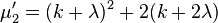
The first few raw moments are:


The first few central moments are:

The nth cumulant is

Hence
Cumulative distribution function[edit]
Again using the relation between the central and noncentral chi-squared distributions, the cumulative distribution function (cdf) can be written as

where  is the cumulative distribution function of the central chi-squared distribution with k degrees of freedom which is given by
-
and where
 is the lower incomplete Gamma function.
The Marcum Q-function can also be used to represent the cdf.[2]
Approximation[edit]
Sankaran [3] discusses a number of closed form approximations for the cumulative distribution function. In an earlier paper,[4] he derived and states the following approximation:

where
-
 denotes the cumulative distribution function of the standard normal distribution;
-

-

-
This and other approximations are discussed in a later text book.[5]
To approximate the chi-squared distribution, the non-centrality parameter,  , is set to zero, yielding

essentially approximating the normalized chi-squared distribution X / k as the cube of a Gaussian.
For a given probability, the formula is easily inverted to provide the corresponding approximation for  .
.
Differential equation[edit]
The pdf of the noncentral chi-squared distribution is a solution of the following differential equation:
![\left\{\begin{array}{l}4 x f''(x)+(-2 k+4 x+8) f'(x)+f(x) (-k-\lambda+x+4)=0 \\[10pt]f(1) 2^{k/2} e^{\frac{\lambda+1}{2}}=\, _0\tilde{F}_1\left(;\frac{k}{2};\frac{\lambda}{4}\right) \\[10pt]\lambda \, _0\tilde{F}_1\left(;\frac{k}{2}+1;\frac{\lambda}{4}\right)+2 (k-3) \, _0\tilde{F}_1\left(;\frac{k}{2};\frac{\lambda}{4}\right)= 2^{\frac{k}{2}+2} e^{\frac{\lambda +1}{2}} f'(1)\end{array}\right\}](http://img.e-com-net.com/image/info8/60825d1d83854eeca25cf884d7348bb5.png)
Derivation of the pdf[edit]
The derivation of the probability density function is most easily done by performing the following steps:
- First, assume without loss of generality that
 . Then the joint distribution of
  is spherically symmetric, up to a location shift.
 - The spherical symmetry then implies that the distribution of
 depends on the means only through the squared length,
  . Without loss of generality, we can therefore take
  and
and  .
. - Now derive the density of
 (i.e. the k = 1 case). Simple transformation of random variables shows that
-
-
-
-
where
 is the standard normal density.
-

- Expand the cosh term in a Taylor series. This gives the Poisson-weighted mixture representation of the density, still for k = 1. The indices on the chi-squared random variables in the series above are 1 + 2i in this case.
- Finally, for the general case. We've assumed, without loss of generality, that
 are standard normal, and so
  has a central chi-squared distribution with (k − 1) degrees of freedom, independent of
  . Using the poisson-weighted mixture representation for , and the fact that the sum of chi-squared random variables is also chi-squared, completes the result. The indices in the series are (1 + 2i) + (k − 1) = k + 2i as required.
Related distributions[edit]
- If
 is chi-squared distributed
  then is also non-central chi-squared distributed:
- If
 and
and  and
and  is independent of
  then a noncentral F-distributed variable is developed as
- If
 , then
- If
 , then
  takes the Rice distribution with parameter
  .
.
- Normal approximation:[6] if
 , then
  in distribution as either
  or
or  .
.
Transformations[edit]
Sankaran (1963) discusses the transformations of the form ![z=[(X-b)/(k+\lambda)]^{1/2}](http://img.e-com-net.com/image/info8/035a2580a8d044248570f6c14939176c.png) . He analyzes the expansions of the cumulants of
. He analyzes the expansions of the cumulants of  up to the term
  and shows that the following choices of
  produce reasonable results:
 makes the second cumulant of approximately independent of
 makes the third cumulant of approximately independent of
 makes the fourth cumulant of approximately independent of
Also, a simpler transformation  can be used as a variance stabilizing transformation that produces a random variable with mean
  and variance
  .
.
Usability of these transformations may be hampered by the need to take the square roots of negative numbers.
| Name | Statistic |
|---|---|
| chi-squared distribution | 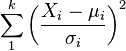 |
| noncentral chi-squared distribution |  |
| chi distribution |  |
| noncentral chi distribution |  |
Occurrences[edit]
Use in tolerance intervals[edit]
Two-sided normal regression tolerance intervals can be obtained based on the noncentral chi-squared distribution.[7] This enables the calculation of a statistical interval within which, with some confidence level, a specified proportion of a sampled population falls.
Notes[edit]
- Jump up^ Muirhead (2005) Theorem 1.3.4
- Jump up^ Nuttall, Albert H. (1975): Some Integrals Involving the QM Function, IEEE Transactions on Information Theory, 21(1), 95–96, ISSN 0018-9448
- Jump up^ Sankaran , M. (1963). Approximations to the non-central chi-squared distribution Biometrika, 50(1-2), 199–204
- Jump up^ Sankaran , M. (1959). "On the non-central chi-squared distribution", Biometrika 46, 235–237
- Jump up^ Johnson et al. (1995) Section 29.8
- Jump up^ Muirhead (2005) pages 22–24 and problem 1.18.
- Jump up^ Derek S. Young (August 2010). "tolerance: An R Package for Estimating Tolerance Intervals". Journal of Statistical Software 36 (5): 1–39. ISSN 1548-7660. Retrieved 19 February 2013., p.32
References[edit]
- Abramowitz, M. and Stegun, I.A. (1972), Handbook of Mathematical Functions, Dover. Section 26.4.25.
- Johnson, N. L., Kotz, S., Balakrishnan, N. (1970), Continuous Univariate Distributions, Volume 2, Wiley. ISBN 0-471-58494-0
- Muirhead, R. (2005) Aspects of Multivariate Statistical Theory (2nd Edition). Wiley. ISBN 0-471-76985-1
- Siegel, A.F. (1979), "The noncentral chi-squared distribution with zero degrees of freedom and testing for uniformity", Biometrika, 66, 381–386
- Press, S.J. (1966), "Linear combinations of non-central chi-squared variates", The Annals of Mathematical Statistics 37 (2): 480–487, doi:10.1214/aoms/1177699531, JSTOR 2238621
External Links[edit]
- Non central chi squared distribution – from itfeature.com