CenterNet做2D和3D目标检测

论文Objects as Points
源码GitHub地址

CenterNet是全卷积的神经网络，不需要额外的NMS的后处理，属于one-stage的检测方法。

1、2D目标检测

通过预测目标的中心点keypoint、由于下采样带来的中心点的偏移offset及尺寸size来获取目标的bounding box。

（1）keypoint: $\hat{Y}$

• 输出的为二值heatmap，$$\hat{Y}\in [0,1{]}^{\frac{W}{R}\times \frac{H}{R}\times C}$$ 1为keypoint，0为background。对于detection，C为类别数。R为下采样率。文中R=4。
  对每个ground-truth keypoint $p$首先计算一个低分辨率的$p=\lfloor \frac{p}{R}\rfloor$， $p$又作用在Gaussian核$$Y_{xyc}=exp(-\frac{(x-p_x{)}^2+(y-p_y{)}^2}{2{\sigma }_p^2})$$
  如果同一类别的高斯核有重叠，选取原则是element-wise maximum。又称为peaks。
• Loss
  Focal Loss
  

（2）offset：$\hat{O}$

• 由于多次下采样带来的目标中心的偏移，$\hat{O}\in R^{\frac{W}{R}\times \frac{H}{R}\times 2}$
• L1 Loss

（3）size：$\hat{S}$

• 预测目标的width和height。$\hat{S}\in R^{\frac{W}{R}\times \frac{H}{R}\times 2}$ ,这里用的就是原始的坐标，没有进行归一化。
• L1 Loss

（4）Bounding Box的计算

$$\begin{gathered} (x-\frac{w}{2}+offset(x),y-\frac{h}{2}+offset(y) \\ x+\frac{w}{2}+offset(x),y+\frac{h}{2}+offset(y)) \end{gathered}$$
x,y为keypoint的预测值，w,h为size，offset(x)和offset(y)为偏移预测。
对于keypoint，文中选取的原则是大于等于与该peaks相连的8个neighbor中的前100个。实现方法为3x3的max pooling。

def _nms(heat, kernel=3):
  pad = (kernel - 1) // 2

  hmax = nn.functional.max_pool2d(
      heat, (kernel, kernel), stride=1, padding=pad)
  keep = (hmax == heat).float()
  return heat * keep

def _topk(scores, K=100):
  batch, cat, height, width = scores.size()
    
  topk_scores, topk_inds = torch.topk(scores.view(batch, cat, -1), K)

  topk_inds = topk_inds % (height * width)
  topk_ys   = (topk_inds / width).int().float()
  topk_xs   = (topk_inds % width).int().float()
    
  topk_score, topk_ind = torch.topk(topk_scores.view(batch, -1), K)
  topk_clses = (topk_ind / K).int()
  topk_inds = _gather_feat(
      topk_inds.view(batch, -1, 1), topk_ind).view(batch, K)
  topk_ys = _gather_feat(topk_ys.view(batch, -1, 1), topk_ind).view(batch, K)
  topk_xs = _gather_feat(topk_xs.view(batch, -1, 1), topk_ind).view(batch, K)

  return topk_score, topk_inds, topk_clses, topk_ys, topk_xs

2、3D目标检测

（1）depth：

• depth直接计算有困难，因此$d=\frac{1}{\sigma (d)}-1\in [0,1]R^{\frac{W}{R}\times \frac{H}{R}\times 1}$.
• L1 Loss

（2）3D dimension

• $dim\in R^{\frac{W}{R}\times \frac{H}{R}\times 3}$
• L1 Loss

（3）orientation

• 用一个标量来回归比较困难。所以选取用8个标量。即$orientation\in R^{\frac{W}{R}\times \frac{H}{R}\times 8}$，一共分了两部分方向角，一个是$[\frac{\pi }{6},-\frac{7\pi }{6}]$，另一个是$[-\frac{\pi }{6},\frac{7\pi }{6}]$，每个方向角用4个标量来表示。其中2个标量用softmax做分类，另外两个做角度回归。
• L1 Loss

3、Human Pose部分，待补充

4、Network

（1）Backbone

detection、pose都用同一个backbone来提取特征。文中选取的Backbone有ResNet18、ResNet101、DLA34、Hourglass104。
其中ResNet18和DLA34采用来DCN（deformable convolution，可形变卷积）,把每个上采样层的3x3的卷积用DCN来替换。

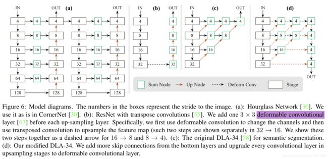
• ResNet：用了3个上采样来提高输出的分辨率，三个上采样层的输出通道分别为256，128，64，在每个上采样之前加了一个3x3的DCN。上采样的卷积核初始化为bilinear interpolation。
• DLA34：skip connection用DCN代替。同样，每个上采样层用3x3的DCN。

（2）Head

在backbone后，接3x3conv-Relu-1x1conv得到网络的输出。
其中3x3conv的channel，对于DLA34是256。

5、Training

• input：512x512
• output：128x128
• data augmentation：random flip and random scaling（from 0.6 to 1.3）,cropping and color jitter。（对3D检测不用data augumentation）
• optimizer：Adam
• ResNet18/DLA34：batch_size=128,8 GPU, lr=5e-4,120epochs，learning rate dropped 10× at 90 and 120 epochs,